Full-hydro simulation of PFI engine using Converge

• Aim:

To perform full-hydro simulation on a port fuel injection engine using CONVERGE and to post process the results using Paraview.

The full-hydro simulation was carried out on a PFI engine geometry for which errors on the surface had been already rectified and no-hydro simulation without any physical models was carried out to check if the simulation runs without error. Now, the full hydro simulation had to be performed with all needed physical models to complete the below objectives;

• Objectives:

1. To calculate compression ratio of the engine.
2. To define the need for using a wall heat transfer model.
3. To calculate the combustion efficiency of the engine.
4. To find the power and torque using engine performance calculator option in CONVERGE.
5. To define the significance of ca10, ca50 & ca90.

• Geometry:

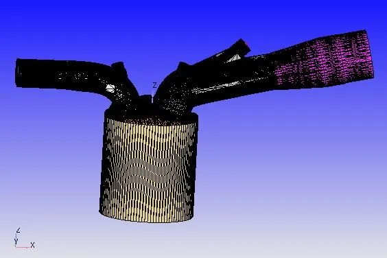
Fig.1 Geometry as .STL file

The surface preparation and boundary flagging had already been completed to test the simulation in no-hyfro mode.

Case setup:

• Application type: Crank angle based

The physical parameters of the engine were as mentoned below;

Bore	0.086 m
Stroke	0.09 m
Connecting rod length	0.18 m
RPM	3000

• Materials:

The PFIengine uses gasoline as fuel. Iso-octane(ICH18) is a fuel which has similar properties to that of gasoline and hence, it was chosen as the parcel species. The thermodynamic data and reaction mechanisms required for the participating species were imported as '.dat' files.

• Simulation parameters:

In case of simulation parameters, full-hydro transient simulation was chosen. The crank angle at the start and end of simulation was set as mentioned below.

Start	-520 deg
End	120 deg

• Boundary conditions & Regions:

The boundaries and regions were assigned to the geometry to run a no-hydro case. The boundary conditions set was as follows;

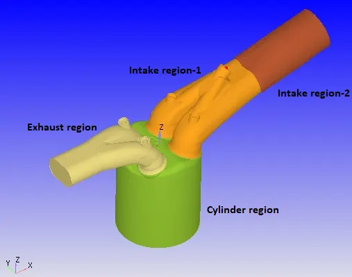
Fig.2 Regions

While assigning the regions, the intake port was split to two(intake region-1 and intake region-2). The regions were split at a location before the fuel injectors. This is done to prevent the flow of fue parcels towards the inflow boundary while the valves are closed. When the valves are closed, the injector will not be injecting new parcels but the fuel parcels from the previous injection may remain in the region and it has to be prevented from moving towards inflow. Also, by splitting the intake region, the initial temperature was specified more accurately since the temperature near the cylinder will be higher than that of the further away,

Boundary name	Region	Boundary type	Boundary motion type	Temperature(K)	Velocity	Pressure(Pa)	Species
Piston	Cylinder region	Wall	Translating, Piston motion	450	Law of wall
Liner	Cylinder region	Wall	Stationary	450	Law of wall
Cylinder head	Cylinder region	Wall	Stationary	450	Law of wall
Spark plug	Cylinder region	Wall	Stationary	550	Law of wall
Spark plug terminal	Cylinder region	Wall	Stationary	600	Law of wall
Exhaust port	Exhaust region	Wall	Stationary	500	Law of wall
Outflow	Exhaust region	Outflow	Stationary	800	Zero normal gradient	101325	CO2= 0.1923, H2O= 0.08855, N2= 0.71913 (mass fractions)
Intake port-1	Intake region-1	Wall	Stationary	425	Law of wall
Intake port-2	Intake region-2	Wall	Stationary	425	Law of wall
Inflow	Intake region-2	Inflow	Stationary	363	Zero normal gradient	101325	Air
Exhaust Valve(top & angle)	Exhaust region	Wall	Translating, user specified motion(exhaust_lift.in)	525	Law of wall
Exhaust valve bottom	Cylinder region	Wall	Translating, user specified motion(exhaust_lift.in)	525	Law of wall
Intake valve(top & angle)	Intake region-1	Wall	Translating, user specified motion(intake_lift.in)	480	Law of wall
Intake valve bottom	Cylinder region	Wall	Translating, user specified motion(intake_lift.in)	480	Law of wall

The exhaust and intake valve motion were specified using an imported lift profile. As mentioned in the above table, the exhaust and intake valves were split into 3 boundaries(top, angle and bottom). This was done for the formation of proper disconnect triangles. Disconnect triangles were triangles formed by Converge to connect two boundaries to replicate closed condition. As it was not possible for two surfaces of different boundaries to intersect each other in converge, it creates disconnect triangles to achieve the connection. For this, while importing the valve lft profile, the min-lift was given as 2e-4 m to specify the minimum distance upto which the valve boundary will come close to the cylinder head to imitate a closed position. At this position, disconnect triangles will be formed between the valve and cylinder head.

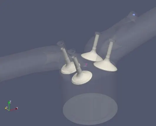
Fig.3 Valve profile

The reason that the disconnect triangles may form incorrectly if the valves were not split as specified in the table was due to the geometry and location of valves at closed position. When the valves are closed, the bottom of the valve will belong to the cylinder while the remaining surface will belong to the intake region. Hence, if the valves were not split into multiples boundaries, it would've been incorrect to assign the entire valve geometry to the intake or the cylinder region.

• Initial conditions:

The initial conditions for the regions were specified as below;

Region	Temperature(K)	Pressure(Pa)	Species(mass fractions)
Cylinder region	1360	185731	CO2(0.1923044025), H2O(0.08855873356), N2(0.7191368639)
Exhaust region	1360	185731	CO2(0.1923044025), H2O(0.08855873356), N2(0.7191368639)
Intake region-1	390	101325	iC8H18 (0.025508), O2 (0.20157), N2 (0.77292)
Intake region-2	370	101325	Air

The initial conditions for exhaust and cylinder regions were considered to be the same as the simulation was set to start by the end of an exhaust stroke. Als, the species mass fractions for the exhaust and cylinder regions were calculated from the stoichiometric composition of the known exhaust species.

Species	Moles	Molecular weight	Mass	Mass fraction
CO2	8	44.01	352.08	0.1923044025
H2O	9	18.01528	162.13752	0.08855873356
N2	47	28.0134	1316.6298	0.7191368639
		Total	1830.84732	1

• Events:

Event type	Region A	Region B	Event	Profile
Cyclic(720 deg)	Cylinder region	Intake region-1	VALVE	Intake valve motion profile(intake_lift.in)
Cyclic(720 deg)	Cylinder region	Echaust region	VALVE	Exhaust valve motion profile(exhaust_lift.in)
Permanent	Intake region-1	Intake region-2	OPEN

The two cyclic events shown in the table correspond to the valve opening and closing events. Since the valves should not come in direct contact with the cylinder head, by setting up events, Converge will create disconnect triangles connecting the valves and cylinder head upon closing. The small distance that separates the valve surface and cylinder head called minimum lift was specified as 2e-4 m. A permanent event was also created to connect the two intake regions. Since they are separate regions, the two regions would not have shared the flow unless specified using events.

• Physical models:

1) Turbulence modelling:

RNG K-epsilon is selected as the turbulence model which is also the default model in converge for the construction and prediction of turbulence.

2) Spray modelling:

Sprays are produced in an engine by high pressure driven liquid(fuel) jets injected into the combustion chamber through injectors with one or more nozzles. The liquid jets are characterized by a dominating direction of motion and atomizes into droplets which evaporates into vapour and upon mixing with air, it forms a combustible mixture which ignites due to increase in pressure and temperature and thus initiates the combustion process. Spray modelling is the prediction and construction of the development of the sprays.

In Converge, two types of injection parameters have to be defined to set up spray modelling: injectors and nozzles. Converge incorporates several models for spray processes including liquid atomization, drop breakup, collision and coalescence, turbulent dispersion, spray-wall interaction and drop evaporation. Converge allows the user to define the spray parcels as spread evenly throughout the spray cone or clustered at the centre of the cone. Since we did not have any data to prove the latter, the parcels were set as distributed evenly in the cone for this case.

Fuel injection: Converge allows the user to define the number of injectors and nozzles required. An injector is a group of nozzles. Also, rate at which fuel is injected can be defined using a normalized plot of the rate profile. The Kelvin-Helmholtz model and Rayleigh-Taylor model were used with recommended constants for gasoline PFI engines to control the breakup of droplets, size of new droplets etc.

Injection time/mass parameters: The start of injection, duration of injection, mass of injected fueland the temperature of fuel had to be defined and was given as follows.

Injection start time(degrees)	-480
Injection duration(degrees)	191.2
Fuel temperature(K)	330
Fuel flow rate(Kg/s)	7.50E-04

The total injected mass per cycle had to be calculated from fuel flow rate per second.

Fuel flow rate(Kg/s)	7.50E-04
RPM	3000
RPS	50
Degree per seconds	18000
Time per degree(s)	0.00005555555556
Time per 720 degree(s)	0.04
Total injected mass per cycle(kg)	3.00E-05

For the simulation, the engine was defined to have one fuel injector with four nozzles. Converge allows the user to set up local coordinate systems, which helps to intuitively configure and manipulate the geometry of the nozzles within an injector.

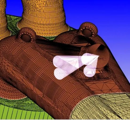
Fig.4 Injector profile

Injection pressure for the sprays was calculated by Converge since only a single value of injection pressure would exist for the provided spray settings like spray duration, rate shape, injected mass etc.

3) Combustion modelling:

A combustion solves the general transport equations for fluid flow and heat transfer as well as the additional equations of combustion chemistry and chemical kinetics. Converge provides detailed chemistry solvers to calculate reaction rates based on the principles of chemical kinetics for accurate prediction of ignition and laminar flame propagation as well as simplified models which are generally less computationally expensive. Simplified combustion models are offered for both premixed and non-premixed combustion and includes CTC/Shell, CEQ, ECFM, ECFM3Z, FGM, G-Equation, and RIF models.

SAGE is a detailed chemistry solver provided by Converge which is widely used for combustion modelling of IC engines. The SAGE model computes the rate of change of species concentration using the Arrhenius equation using the reaction mechanism data provided by the user. Since SAGE is a detailed chemistry solver, solving for the entire domain is computationally expensive. Hence, Converge provides options to define the start/end time, regions, minimum cell temperature and species mole fractions to lower the number of cells in which combustion calculations are carried out. Furthermore, Converge includes multi-zone modelling which groups individual cells into zones based on variables like temperature, reaction ratio etc and invokes SAGE to calculate the average quantities per zone instead of per cell, thus speeding up the calculations.

SAGE parameters provided for the present PFI case was as below:

Start	-17 deg
End	130 deg
Minimum cell temperature	600K
Minimum HC species mole fractions	1.00E-08

4) Source/Sink modelling:

Source modelling is required to set up energy source over the spark plug for ignition. This energy source increases the temperature of species adjacent to it and this temperature change would be introduced in the species transport equations thus affecting its chemical kinetics and further reactions leading to further increase in temperature. For the present case, spherical energy sources were created at the spark plug terminal location. The spark parameters were set as shown below;

Start of spark	-15 deg
End of spark	-5 deg
Energy	0.02 J

In addition to the above source, another spherical source was also set up with the same energy input. But the duration of this new source was set to only 0.5 degrees. The reason for providing additional energy in the initial 0.5 degrees of spark is to reproduce the energy input of a real spark ignition as per experimental data.

• Grid control:

1) Base grid:

A base grid of 4 mm was set for the simulation

2) Fixed embedding:

Fixed embedding is a mesh refinement technique in Converge to refine the mesh at a pre-defined location as desired by the user. The location for embedding can be specified by boundary, region or by creating geometrical shapes over the required area. The refinement is done by scaling the base grid by powers of 2. The following embeddings were set up for the present case.

Entity type	Boundary/ Location	Mode	scale	Star time(deg)	End time(deg)
Boundary	Intake valve angle	Permanent	3	-	-
Boundary	Exhaust valve angle	Permanent	3	-	-
Cylinder	Cylinder zone	Permanent	1	-	-
Cylinder	Cylinder zone	Permanent	2	-	-
Sphere	Spark plug zone	Cyclic (720 deg)	5	-16	7
Sphere	Spark plug zone	Cyclic (720 deg)	3	-16	7
Injector	Injector	Cyclic (720 deg)	4	-480	-286

3) Adaptive Mesh Refinement(AMR):

Adaptive mesh refinement is an autonomous meshing option in Converge which creates the mesh at run time and dynamically adapts it throughout the simulation to maximize both computational efficiency and accuracy. AMR can automatically adjust the grid as needed at each time-step, adding cells at areas of interest and removing cells at areas where it is not necessary. Converge achieves this by monitoring changes in parameters like velocity, temperature, species etc. By doing so, AMR refines cells were complex phenomena are occurring while ignoring areas where no noticeable changes occur. The refinement is done as per sub-grid scale(SGS) provided by the user. The grid is scaled as per the below equation;

Refined cell size = `(Base grid size)/2^(SGS)`

Thus, a higher value of SGS will give high refinement. The AMR setup for the present case was as below;

AMR type	Max. embedding level	Sub-grid criterion	Timing control	Star time(deg)	End time(deg)
Velocity	3	1	Permanent	-	-
Temperature	3	2.5	Cyclic (720 deg)	-17	135

Observations & Results:

The simulation ran successfully. The results obtained were as follows;

• Meshing:

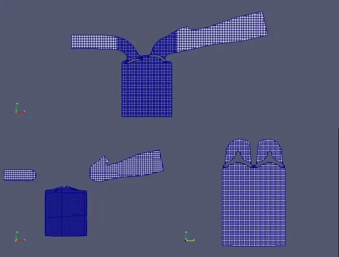
Fig.5 Mesh view

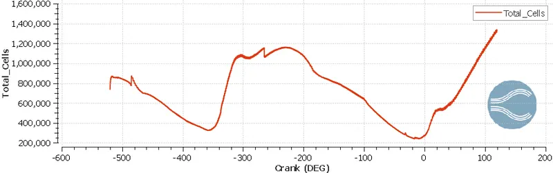
Plot.1 Cell count

The max cell count was recorded as 1340000 during the simulation.

• Simulation animation with engine surface coloured by temperature

The simulation starts by the beginning of intake stroke and ends by exhaust stroke.

• Temperature changes inside the cylinder

The change in temperature inside the combustion chamber due to spark ignition and combustion can be seen in the above animation.

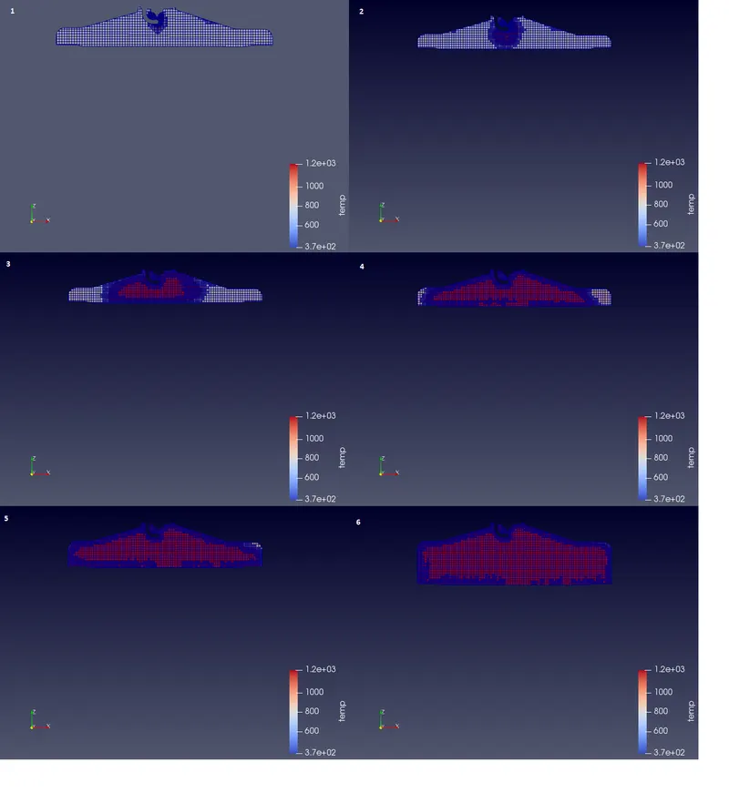
Fig.6 Spark ignition

The initiation of spark can be seen in the first cut plane. As the spark was initiated, the mesh in the region was refined thanks to adaptive mesh refinement(AMR). With further propagation of the flame, the mesh can be seen getting refined.

• Compression ratio:

Compression ratio of an engine is the ratio of cylinder volume when the piston is at the top and bottom of its travel. The force which compresses the air-fuel mixture inside the combustion chamber to create ignition depends on the compression ratio i.e, the volume of the cylinder when the piston is at the bottom of its stroke versus the volume of the cylinder when the piston is at the top of its stroke. Every engine has a specific compression ratio. Compression ratio is given by the below equation;

CR= `(V_d + V_c)/V_c`

Where, `V_d` is the displacement volume or the volume inside the cylinder that is displaced by the piston from beginning to end of compression stroke and `V_c` is the clearance volume or the volume left in the cylinder at the end of compression stroke.In the above equation, `(V_d + V_c)` is the peak volume inside the cylinder and `V_c` the minimum volume in the cylinder. Hence, compression ratio can be easily found from the volume chart of the given PFI engine.

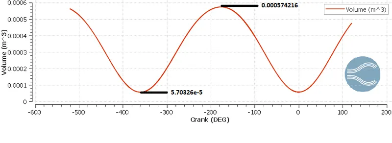
Plot.1 Volume changes inside combustion chamber

Maximum volume inside cylinder = 0.000574216 `m^3`

Minimum volume inside cylinder= 5.70326e-5 `m^3`

Therefore, CR = `0.000574216/(5.70326e-5)` = 10.068

The compression ratio of given PFI engine was found to be 10:1.

• Combustion efficiency:

Combustion efficiency is the ratio of energy released by the burnt fuel to the theoretical energy content of the fuel mass in a single cycle. If there is excess fuel or lack of air it would result in incomplete combustion of a fraction of fuel. Therefore, combustion efficiency is an important term which measures the engine's ability to convert the input energy(fuel) into heat energy.

To calculate combustion efficiency, we need to know the energy content of the fuel mass injected and heat released in one complete cycle.

Combustion efficiency, CE = `(H_R(T_A)-H_P(T_A))/(m_f*Q_(HV))`

Where,

H_R [J] – enthalpy (internal energy) of the reactant
H_P [J] – enthalpy (internal energy) of the product
T_A [K] – ambient temperature
m_f [kg] – mass of fuel injected per cycle
Q_HV [J/kg] – lower heating value of the fuel

The numerator in the above ratio is the actual heat released by the input fuel during combustion. This can also be found from the peak value of integrated heat release rate.

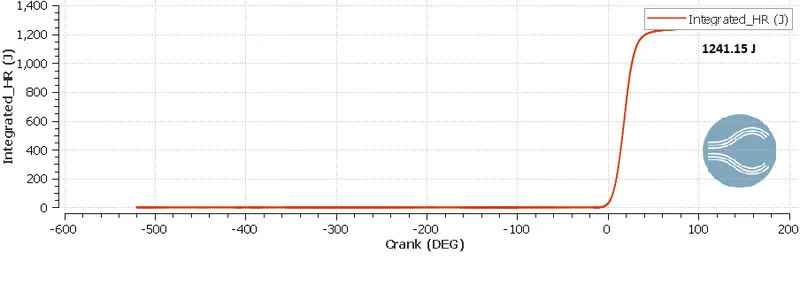
Plot.2 Integrated heat release rate inside combustion chamber

Peak integrated heat release rate = 1241.15 J

Mass of fuel per cycle,`m_f` = 3.0e-5 kg

Lower heating value of fuel(iso-octane) = 44.651 MJ/Kg = 44651000 J/Kg

Therefore, CE = `1241.15/((3e-5)*44651000)` = 0.926

The combustion efficiency of the engine was found to be 92.6 %

• Determination of power and torque:

Power:

Power is the work done per unit time. In Converge line plotting module, Converge provides a calculator which is capable of calculating various data on the engine performance. The engine performance calculator gave the following results;

The work done for combustion was obtained as 468.646 Nm.

Total duration of combustion = 240.199 degrees

RPM = 3000

RPS = 50

Degrees per second, DPS = 50*360 = 18000

Total duration of combustion(in seconds) =`240.199/18000 = 0.01334 s`

Therefore, Power = `468.646/0.01334 = 35130.88`J/s = 35.13 KW

Torque:

The rotating power produced by the engine's crankshaft is known as Torque. It is also the ability of the engine to perform work.

Since, Power(P) = `(2*π*N*T)/60` = 35130 W;

Where, RPM = 3000 rev/min

Then, Torque(T) = `(P*60)/(2pi*N)` = `(35130*60)/(2*pi*3000)`= 111.82 Nm

• Combustion chamber parameters:

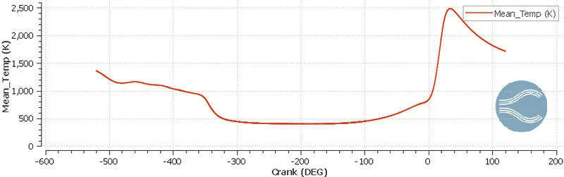
Plot.3 Temperature changes inside combustion chamber

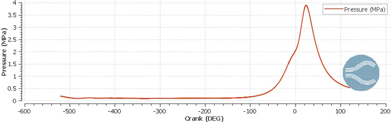
Plot.4 Pressure changes inside combustion chamber

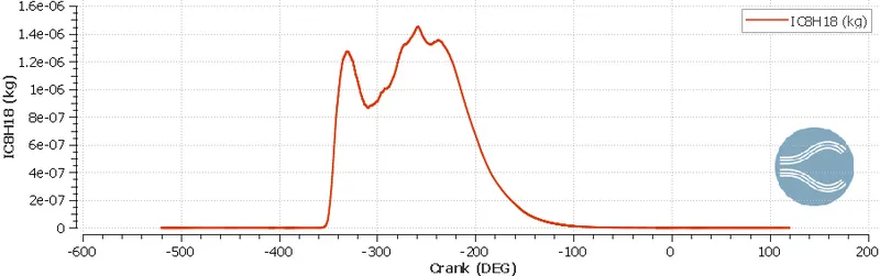
Plot.5 Fuel species mass inside combustion chamber

• Emissions parameters:

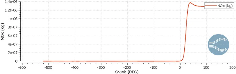
Plot.6 NOX emissions

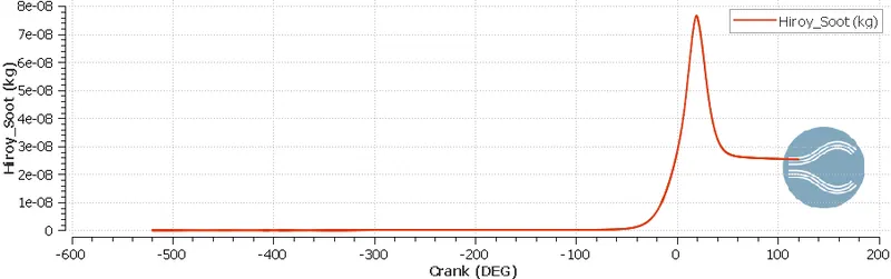
Plot.7 Soot emissions

• Need for wall heat transfer model:

In CFD simulations, solid wall boundaries are usually treated as adiabatic since Navier- Stokes equations are only concerned with fluid flow and cannot solve for solid heat transfer.Hence, walls are considered as voids and do not take part in the transfer of heat. In the current simulation, when combustion occurs inside the chamber, the generated heat was not transferred to the engine block since the walls were treated as adiabatic. But in actual cases, when the temperature rises inside the chamber, the heat is transferred to the liner by convection and then to the engine block by conduction. Since the leaked heat energy affects the efficiency of the engine negatively it is essential to take account of energy loss due to wall heat transfer to get realistic results. Conjugate heat transfer analysis allows for simulation of heat transfer between fluid and solid domains by exchanging thermal energy at the interfaces between them.

• Significance of CA10, CA50 and CA90:

The terms CA10, CA50 and CA90 signifies the crank angle at which a certain percent of total injected fuel mass has been burned or the position of the crank angle(deg) at which the cumulative heat release reaches at 10%, 50% and 90% respectively. In Converge, this data can be obtained from the engine performance calculator option in the line plotting module. For the present case, the following results were obtained;

CA10(deg)	CA50(deg)	CA90(deg)
6.83717	18.4623	31.701

Apart from denoting the heat release percentage, they also provide other insights. CA10 denotes the start of ignition in a diesel engine and the difference between start of fuel injection and CA10 is identified as ignition delay. CA50 indicates the end of premixed combustion and the start of diffusion combustion of fuel used in the engine. The difference between CA90 and CA10 gives the combustion duration as well.

Conclusion:

Ran the simulation successfully using Converge and post-processed the results using Paraview and Converge line plotting module. Created animations and plots and analyzed the results.