ODE stability literature review

• Aim:

To study stabilty of ordinary differential equations and its effect on engineering simulations.

An ordinary differential equation(ODE) is an equation that involves ordinary derivatives of one or more functions of an independent variable. To solve an ODE implies to determine what function or functions satisfy the equation.

Although many differential equations cannot be solved using analytical methods, for engineering applications, numerical integration methods are used to get approximations to the solution of ODEs. One of the classifications of these numerical integration methods are as explicit and implicit methods. Euler method is an example for explicit numerical method and Backward Eulermethod is an example for an implicit numerical method.

An ODE function f(x) is said to be stable if the solutions of the equatoin remains close to each other for succeeding values of x. If the difference between the solutions approaches zero as x increases, the solution is called asymptotically stable. If a solution does not have either of these properties, it is called unstable. If the solution remains stable for arbitrarily large step sizes, the method is unconditionally stable.

While using explicit method for approximating solution, certain ODEs turn unstable. These can be charaterized as stiff equations that includes some terms that can lead to rapid variation in the solution. These ODEs cannot be solved using explicit metod unless the step size is taken to be extremely small. Implicit methods are usually more stable for solving a stiff equation, meaning that a larger step size can be used, although not always unconditionally stable.

The stability of an ODE can be illustrated by calculating the solution for the below mentioned ODE using analytical method, explicit method and implicit method.

`dy/dt = -1000y - e^(-t)`

The equation can be modied to solve using the above mentioned 3 methods as shown below.

• Analytical method:

`y(t) = (e^(-1000t)(1-e^(999t)))/999`

• Explicit method

`(y^(n+1)-y^n)/dt = -1000y^n- e^-t`

`y^(n+1) = y^n - (1000y^n+ e^-t)dt`

• Implicit method

`(y^(n)-y^(n-1))/dt = -1000y^n- e^-t`

`y^n= (y^(n-1)-e^(-t)dt)/(1+1000dt)`

• Python code:

import matplotlib.pyplot as plt
import numpy as np 
import math as mt
'''
ODE : dy/dt = -1000y - e^(-t)

Analytical method:
y(t) = (e^(-1000t)(1-e^(999t)))/999

Explicit method:
y^(n+1) = y^n - (1000y^n+ e^-t)dt

Implicit method:
y^n= (y^(n-1)-e^(-t)dt)/(1+1000dt)
'''
total_t = 0.1
dt = 1.99e-3
t = np.arange(0,total_t,dt)
y = np.zeros(len(t))

def analytic(total_t,t):
	t = np.arange(0,total_t,dt)
	y = np.zeros(len(t))
	for i in range(1,len(t)):
		y[i]= (mt.exp(-1000*t[i])*(1-mt.exp(999*t[i])))/999
	return [t,y]

def explicit(total_t,t):
	t = np.arange(0,total_t,dt)
	y = np.zeros(len(t))
	for i in range(1,len(t)):
		y[i]=y[i-1]-(1000*y[i-1]+mt.exp(-t[i-1]))*dt
	return[t,y]

def implicit(total_t,t):
	t = np.arange(0,total_t,dt)
	y = np.zeros(len(t))
	for i in range(1,len(t)):
		y[i]=(y[i-1]-(mt.exp(-t[i-1]))*dt)/(1+1000*dt)
	return[t,y]

t,y_explicit = explicit(total_t,t)
t,y_implicit = implicit(total_t,t)
t,y_analytic = analytic(total_t,t)
plt.plot(t,y_explicit,'b',label='Explicit')
plt.plot(t,y_implicit,'g',label='Implicit')
plt.plot(t,y_analytic,'r',label='Analytic')
plt.legend()
plt.show()

• Plots:

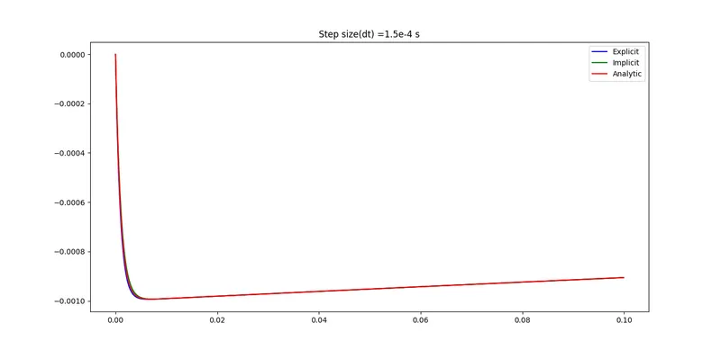
Plot.1

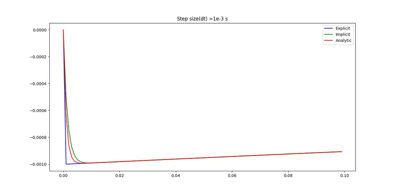
Plot.2

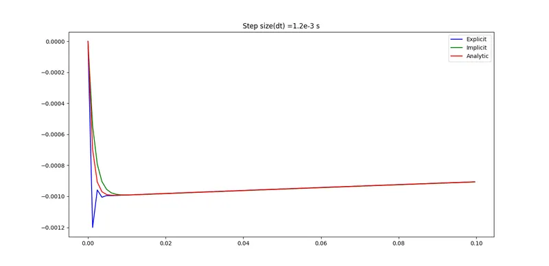
Plot.3

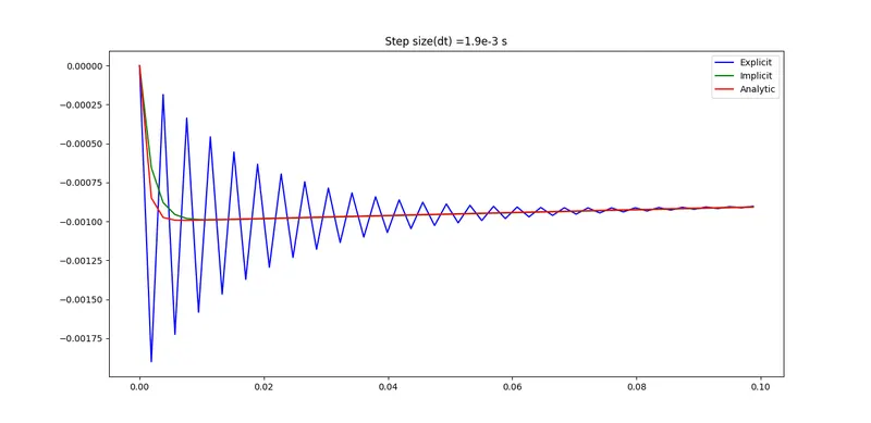
Plot.4

• Observations:

The above four plots were taken successively with increasing value of step size 'dt'. It is evident that the explicit method becomes highly unstable after a small increase in the step size. Although the implicit method gavea smooth plot, compared to the analytical answer, a slight variance can be noted. But when compared to the explicit method, the line plot of implicit method made far more sense and was much closer to the exact answer.

Since stability of an ODE is crucial to obtain accurate values, an unstable solution will certainly give inaccurate results. For engineering simulations, a small error may be inevitable while approximation, but if the ODE gives unstable results, the solution cannot be considered as valid and should be discarded.

Every Problem thats needs solving is based on an expression of some form or another. It is important to know that the expression is continuous in its inputs, so that the results would not becompletely different for slight changes in input. To have confidence in the solution, the expression must also be well conditioned. A well conditioned expression will give small changes in results for small changes in the input. If the solution is unstable and leads to large change in output, then the problem can be classified as ill-conditioned. The exact cut-off between well conditioned and ill-conditioned depends on the context of the problem and the uses of the results.