Prandtl Meyer Shock study using Converge CFD

Aim:

• To run a Prandtl-Meyer shock problem using Converge CFD and post process the results using paraview.

Objectives:

• To define Shock waves.
• To explain typical boundary conditions used for shock flow problems.
• To run a prandtl Meyer shock problem with CONVEGRE and study the effect of SGS criterion of CONERGE on shock location.

Shock waves:

When the local flow speed exceeds the local sound speed, the continuity of flow is abrupted. This disturbance is characterized by instantaneous change in pressure, density, flow velocity, temperature and Mach number. This kind of propagating disturbance is known as shock wave and it carries an energy like an ordinary wave.

Shock flow boundary conditions:

Generally in shock flow problems, shear stress and boundary layer formation is undesired as the objective of the problem is revolving around the shock formation. Hence, free slip boundary conditions are used at walls so that they may not influence the flow. Slip boundary condition enables the flow of fluid relative to a wall hence effect of solid boundary on fluid flow will not be considered. For properties such as pressure, velocity or temperatur, Neumann boundary conditions are usually applied unless value is to be specified.

Geometry;

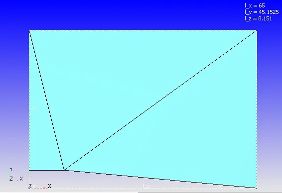
At the bottom of the geometry, the wall is tilted at almost `10^0` downwards after a distance from inlet. When flow encounters this convex shape at supersonic speeds, shock waves are likely to be generated.

Setup:

• Application type: Time based
• Material: Air
• Solver: Steady state pressure based PISO scheme solver
• Boundary conditions:

1) Inlet: Inflow boundary

Velocity = 680 m/s

Pressure: Zero normal gradient boundary

2)Outlet: Outflow boundary

Velocity & pressure: Zero normal gradient boundary

3) Front & back: 2D boundary

4) Top and bottom walls: Slip boundary

• Initial conditions:

Species: O2 & N2

• Turbulence model: RNG K-epsilon
• Grid control:

In grid control, adaptive mesh refinement(AMR) was enabled so as to refine the mesh at locations where shock waves are expected to be formed. As the temperature changes instantaneously during shock waves, AMR was set based on temperature. It will locate changes in temperature in cells and refine the mesh based on the sub grid scale(SGS) criterion given.

Base grid = 0.8 m

Adaptive mesh refinement(temperature):

Case.1 SGS criterion = 0.05

Case.2 SGS criterion = 0.03

For most of the part the default values were used for setting up this simulation. The simulation was set to run for 25000 cycles.

Results and observations:

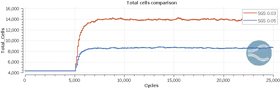
Plot.1: Total cell count comparison with respect to SGS criterion.

It can be seen from the above plot that after 5000 cycles, the cell count began to rise for both cases as adaptive mesh refinement was set to begin after 5000 cycles. Also, a significant difference in cell count can be seen while comparing both cases. The cell count for SGS criterion 0.03 was nearly 7000 units more than 0.05 case.

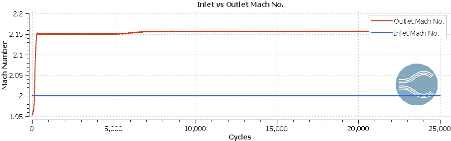
Plot.2: Mach number comparison, Inlet vs Outlet.

It is evident from the plot that fluid moves at supersonic speeds inside the domain as Mach number is greater than one at inlet and outlet. Also, outlet mach number is higher implying flow velocity at outlet is greater compared to inlet.

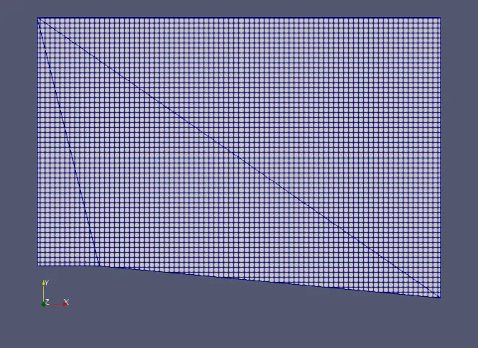
Fig.1:Initial mesh

The initial mesh was noted to be just over 4000 cells.

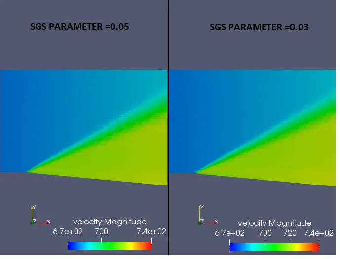
Fig.2:Final velocity contour

In the above figures, it can be seen that along a line, beginning from a point at the curvature in the geometry, the velocity begins to rise. The velocity acceleration is happening in a fan like shape gradually spreading as it moves further away from the origin. This phenomenon is known as Prandtl Meyer expansion fan. It occurs because it is physically impossible for the flow to turn through a single "shock" wave because this would violate the second law of thermodynamics. The flow velocity rises as it turns around at the corner and stabilizes later. It can be noted that the velocity contour obtained from SGS criterion 0.03 is a bit more resolute than SGS 0.05.

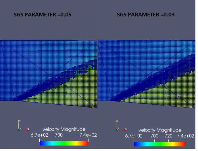
Fig.4: Final mesh comparision with respect to SGS parameter

The above figure compares the cell formation for the two different cases that was run. As the adaptive mesh refinement was set for temperature change, the refinement can be seen at the expansion fan where the shock waves are generated. The shock waves result in lowering of temperature. The SGS criterion notes this change and refines the mesh at the region accordingly. From the figure it is evident that for a lower value of SGS criterion, a higher refinement of the region was achieved. The countour plots of the lower SGS criterion(0.03) case was much more refined than that of the other.

Simulation Animations:

1) SGS criterion 0.05

2) SGS criterion 0.03

Conclusion:

Successfully ran Simulation for Prandtl Meyer shock problem using CONVERGE Studio and post processed the results using PARAVIEW. Utilized the adaptive mesh refinement tool to get refined results. Created contours showing the prandtl Meyer expansion fan. Familiarized with shock waves and common boundary conditions used for shock wave problems.