Transient simulation of flow over a throttle body
Aim:
To Simulate flow over a throttle body using Converge CFD.
A throttle body is a butterfly valve usually located between the air intake filter and the intake manifold in an engine. It regulates the amount of air going into the engine. The amount of airflow into the engine cylinder depends on the butterfly valve angle. The angle at which the butterfly valve has rotated also has an effect on the mixing efficiency of air and fuel as vortexes are generated in the wake of flow over the throttle.
CONVERGE Studio and Paraview softwares were used to run and post-process this simulation. In this analysis, the valve angle is changed from `0^0` to `25^0` where `0^0` being fully open. The throttle body under study here is inside a pipe elbow consisting of three boundaries ie, inlet, outlet and wall. The inflow fluid pressure was specified for inlet boundary and static pressure specified for outlet boundary.
Geometry:
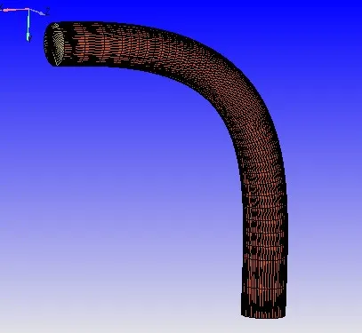
Fig.1 Pipe geometry
The throttle valve is situated midway inside the elbow initially in open condition.
Throttle valve geometry:
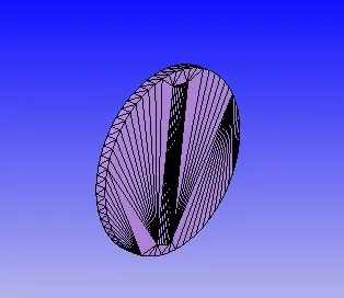
Fig.2 Throttle geometry
SETUP:
- Application type: Time based
- Solver: Transient
- Total simulation run time:
The total run time for the simulation had to be calculated so that enough fluid may pass through the domain to get a meaning ful output. To calculate the same, the basic velocity formula was used.
v = d/t where, v= inlet velocity, d= distance travelled by fluid, t= time.
here, distance travelled by the fluid equals the total length of the pipe, which roughly equates to 0.2 m found from measruing the geometry.
The inlet velocity of flow was found by running the simulation in steady state condition for the same boundary conditions. Velocity was found to be equal to 193 m/s
hence, Time, t= 0.2/193 = 0.001 seconds.
This time is the time it takes for the fluid particles to pass the entire lenght of pipe once. To get a meaningful result, the time for the fluid to flow atleat ten times was considered.
Hence, total flow time = 0.001*10 = 0.01 seconds.
- Initial time step: 1e-9 seconds
- CFL values: default values
- Solver parameters: PISO scheme with pressure based solver type
- Boundary conditions:
1) Inlet: Inflow boundary
Pressure = 1.5 bar
2) Outlet: Outflow boundary
Pressure = 1 bar
3) Pipe wall: Wall boundary
4) Throttle valve: Wall boundary
To simulate the movement of the walve, the wall movement type was set to 'rotating' and surfave movement to 'moving'. The axis and center of rotations were entered. Afile was used to define the movement of the throttle. It was set in a manner that the throttle would turn `25^0` from `0^0` and later return to `0^0`.
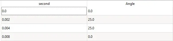
Table.1 Throttle rotation rate file
- Initial conditions(inside flow region):
Species: O2, N2
Temperature: 300K
Pressure: 101325 Pa
Velocity 0 m/s
- Turbulence model: RNG K-epsilon
- Grid/Meshing:
The base grid was given as 2mm in all directions. Fixed embedding was enabled at throttle wall boundary to refine mesh at the area. The figure below is of a cutplane of the geometry with the mesh visible.
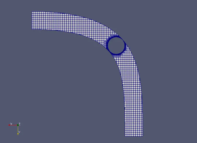
Fig.3 Meshing
Results and observations:
The simulation ran successfully for 0.1s.
- Total cell count:
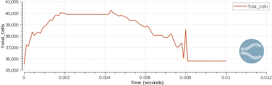
Plot.1 Cell count
It can be seen that the initial cell count of 35000 rose upto 40000 when the throttle turned `25^0` and later returned to initial value at `0^0` throttle angle.
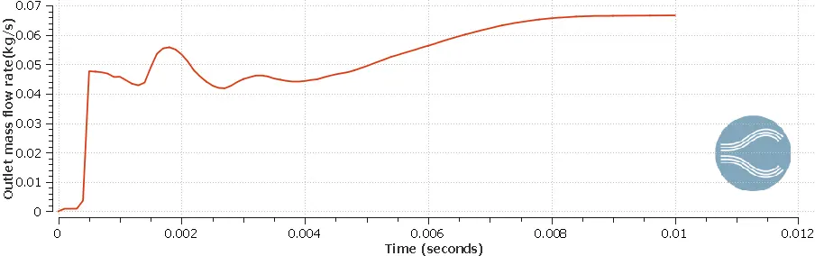
Plot.2 Outlet mass flow rate.
The mass flow rate can be seen decreasing as throttle started to close the flow area. The flow rate later reached a steady value of 0.06kg/s after the throttle returned to fully open condition.
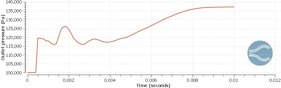
Plot.3 Outlet Pressure.
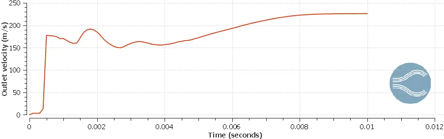
Plot.4 Outlet Velocity.
From the pressure and velocity plots, a pattern similar to mass flow rate plot was observed.
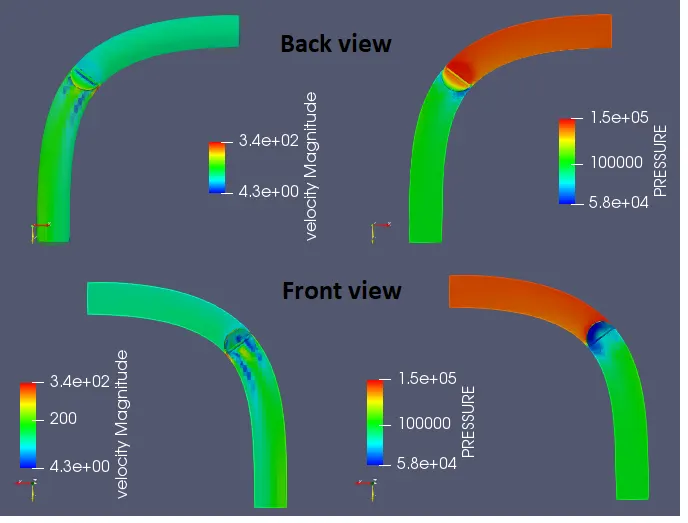
Fig.4 Pressure & Velocity Contours at `25^0` throttle angle. Throttle also visible.
The above contours were taken at `25^0`angle of throttle. In the velocity contour, a wake can be observed behind the throttle. The flow got irregular for a short distance after the throttle. The pressure was increased in the area preceding the valve owing to constriction of flow path. A low prressure region is formed behind the valve where the wake is situated.
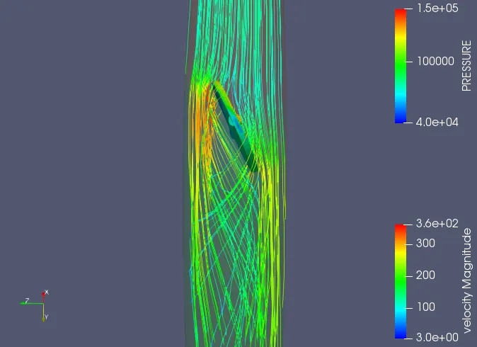
Fig.5 velocity stream lines & throttle with pressure contour.(side view)
From the above figure, the vortex formation behind the throttle valve can be observed in clarity. The velocity rises when it passes through the consrticted path of flow near throttle. A stagnation area was observed in the frontside of the throttle valve where the velocity is near zero while pressure is the highest. The flow has been brought to rest by the throttle valve surface in thre frontal area.
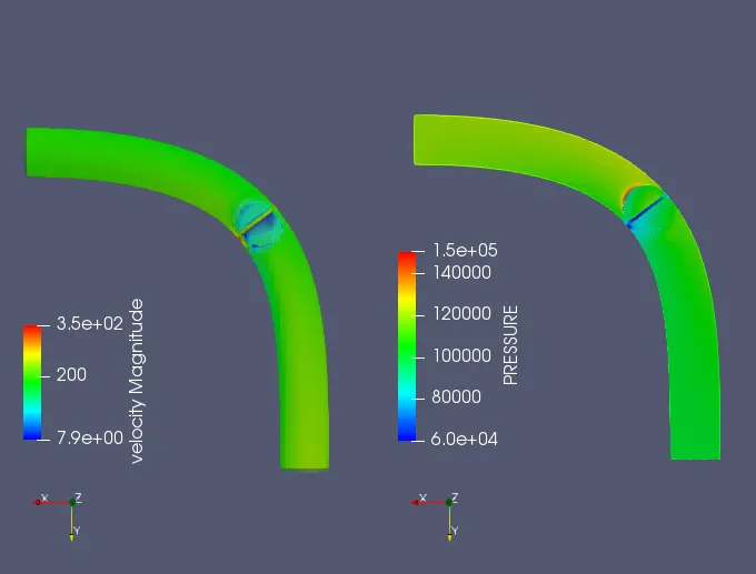
Fig.6 Final Velocity & Pressure contour.
The above figure shows velocity and pressure distribution after 0.01s of flow. The throttle is fully open at the moment. The magnitudes of velocity and pressure are fairly uniform as there is minimal resistance to flow.
Flow Animation:
Conclusion:
The simulation of flow over a rotating throttle body was successfully completed and analyzed the results. The restriction to flow created by the throttle body resulted in irregularities in the flow. The vortex generated by the wake region formed succeeding the throttle reduces the velocity of the fluid and also would have an effect on mixing efficiency had there been multiple fluids. The stagnation point was observed to be at the front face of the butterfly valve while negative pressure area was observed in the wake region.