Week-6 Calculate the Stretch Ratio by comparing the ELFORM (-2,-1,1,2) with Ogden_Material Model.

WEEK-6

AIM

• To create a block of 10*10*10 mm dimensions of elements in each direction and to assign a given Odgen material with material properties.
• use appropriate boundary conditions to simulate a tensile test of a model using different ELFORMS(1,-1,2,-2).
• Calculate true stress, true strain along with engineering stress & engineering strain with a stretch ratio for all the ELFORM in excel sheet.
• Finally, compare the image plots of all ELFORMS against the uniaxial plot and summarize the results.

INPUT DATA

• ogden_Material.k
• block of 10*10*10 mm dimensions of elements
• ELFORMS (1,-1,2,-2)
• STRETCH RATIO λ = (1+Engineering strain)
• Uniaxial plot

OUTPUT DATA

• An excel sheet with proper conservation & calculation of stress/strain & stretch ratio for all ELFORM
• A Plot image with various comparisons of ELFORMS against the uniaxial plot and summarize the simulation results.

PROCEDURE

• Initially, open the LS-PRE POST and open the ogden_Material.k file
• Go to elements and mesh → shape mesher → create block of 10*10*10 mm dimensions of elements in each direction

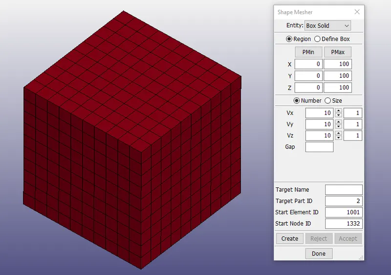
Fig, represents the creation of solid elements with 10*10*10 mm dimensions in X, Y & Z direction

• Go to the section and assign a section solid and assign ELFORM 1 for the solid section.

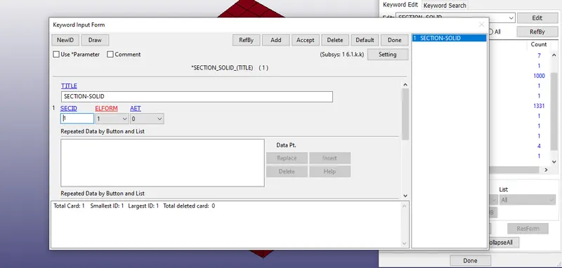
Fig, represents the assignment of ELFORM 1 to the solid section

• once, the section is created go to the part and assign the section and material ID for the part

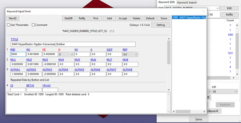
Fig, represents the Ogden material with material properties

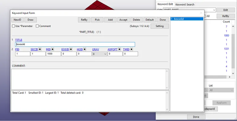
Fig, represents the assignment of Material & secttion ID to the part

• Then, the displacement curve is defined by define → curve option.
• The stretch ratio is calculated by using a formula, λ = (1+dL/L0)

λ = 5

5=(1+dL/10)

dL=40 , L=dl+L = 40 +10=50

• The displacement & time are assigned in the curve along with the termination time.
• An extra time is provided to avoid instabilities and to avoid warning issues.

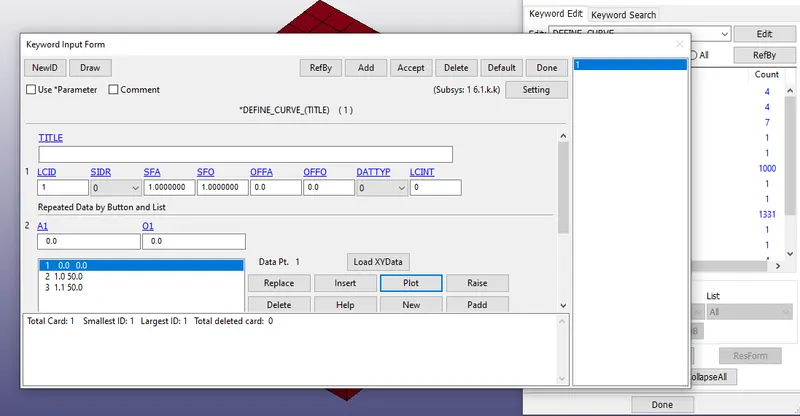
Fig, represents the assignment of time step values and displacement in the curve

• The curve is plotted to check whether the assigned values are plotted successfully or not.

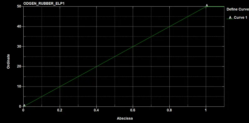
Fig, represents the variation of displacement over the period of time (Disp vs time)

• Then, the next step is to assign the boundary conditions in order to simulate the tensile test model for that, go to create entity option → set node→to pick the set of nodes in the x-direction

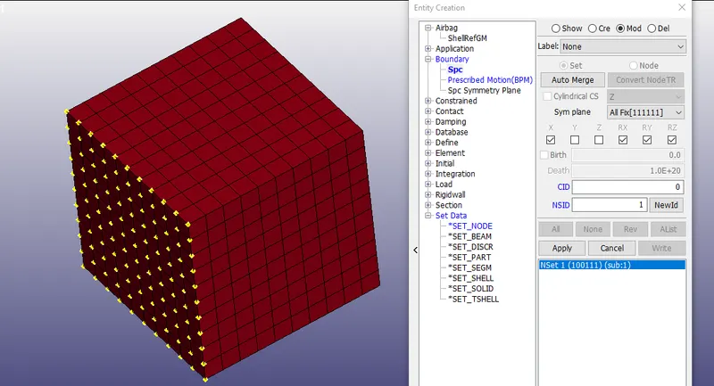
Fig, represents the picking the set of nodes in the X direction

• The nodes are constrained in the x-direction, RX , RY and RZ and in the other hand the nodes are allowed to move free in the Y and Z direction respectively.

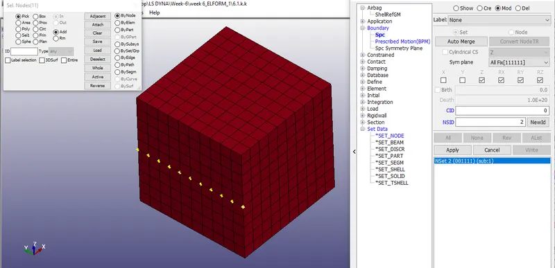
Fig, represents the picking the set of nodes in the Y direction

• The nodes are constrained in the Y-direction, RX , RY and RZ and in the other hand the nodes are allowed to move free in the X and Y direction respectively.

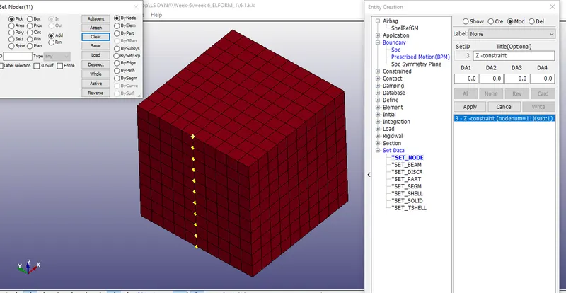
Fig, represents the picking the set of nodes in the Z direction

• The nodes are constrained in the Z direction, RX , RY and RZ and in the other hand the nodes are allowed to move free in the X and Z direction respectively.
• These boundary conditions are given to see the effect of the Poisson ratio or Poisson effect when the tensile or displacement is given in the X-direction.
• When the displacement is given the nodes have to move freely in the direction perpendicular to it. i.e when the displacement is given the material has extended in the x-direction and it has to compress in the y and z direction respectively and in order to achieve this behavior the boundary conditions or the constraints are given in the x,y and Z direction respectively.
• Then finally, NSID is created to assign the displacement in the x-direction.

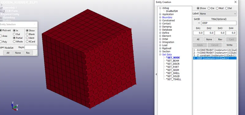
Fig, represents an NSID is created for the assignment of Displacement in the X-direction.

• After, assigning the NSID for displacement a boundary prescribed motion is set is selected in the keyword manager → boundary → boundary prescribed motion set
• After, that the NSID and displacement are assigned in the boundary prescribed motion set to initiate the displacement at the nodes in the x direction.

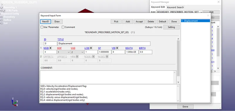
Fig, represents the assignment of NSID and displacement in the boundary prescribed motion set

• Finally, in the control card, the energies for various HGEN, RWEN, SLTEN, RYLEN,IRGEN is assigned to compute various energies in the output.

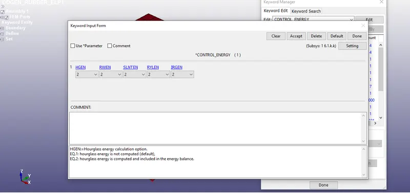
Fig, represents the assignment of various energies in the *control energy card

• Then, implicit auto is selected in the control card, this is done to ensure the implicit solver calculated the number of iterations that give to ITEOPT value and ITEWIN
• This is generally done to calculate the optimum number of iterations that we need to solve for every time step and we give a value to ITEWIN to adjust the convergence in accordance with it.
• Finally, we assign a termination time to end the problem and we here assign the value as 1ms.
• The same procedure has been repeated for different ELFORMS (-1,2-2)
• The previous.k file which has ELFORM 1 is been edited in Notepad++ and we change the ELFORM to -1 in the section solid.
• The same procedure has been done for changing different ELFORMS.

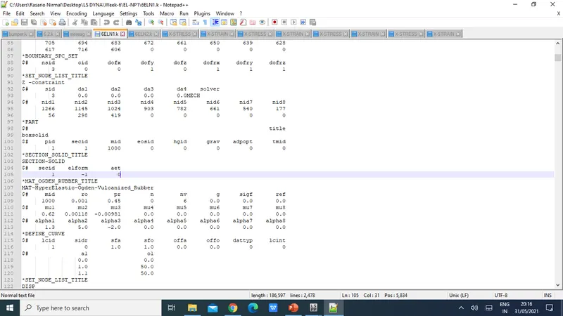
Fig, represents the changing of ELFORM to -1 in the section solid.

• Finally, the ogden_Material.k containing different ELFORMS has been opened in LS - RUN and terminated successfully.

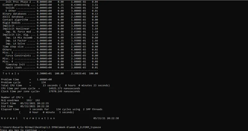
• The reason why choose, the implicit solver to compute the problem is that the implicit solves the problem with greater accuracy and ensures the force equilibrium at each time step that we provided. Additionally, it provides the stability to the model during the computation. Furthermore, since it provides greater accuracy to the model by solving and forcing the problems to ensure the equilibrium conditions and in that aspect, we consider in choosing the implicit solver to compute the problem.

RESULTS

FINAL ANIMATION OF X STRESS FOR ELFORM (1,-1,2,-2)

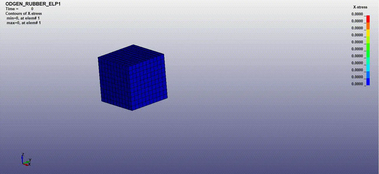
Fig, represents the X-STRESS ANIMATION of OGDEN MATERIAL with ELFORM1

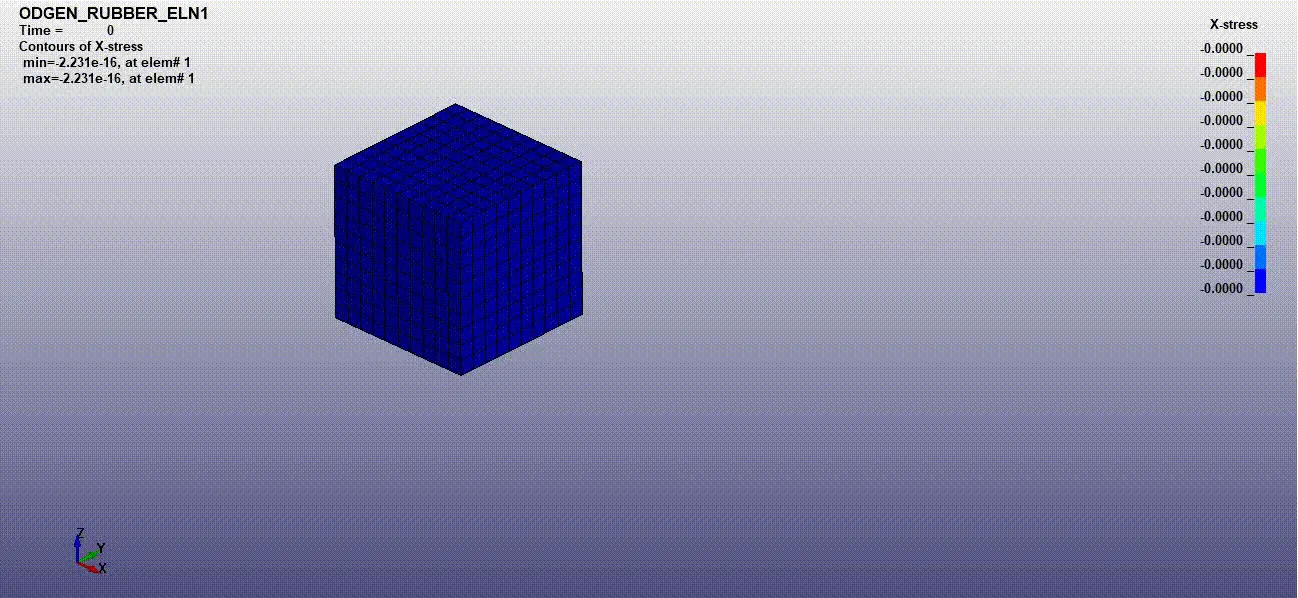
Fig, represents the X-STRESS ANIMATION of OGDEN MATERIAL with ELFORM-1

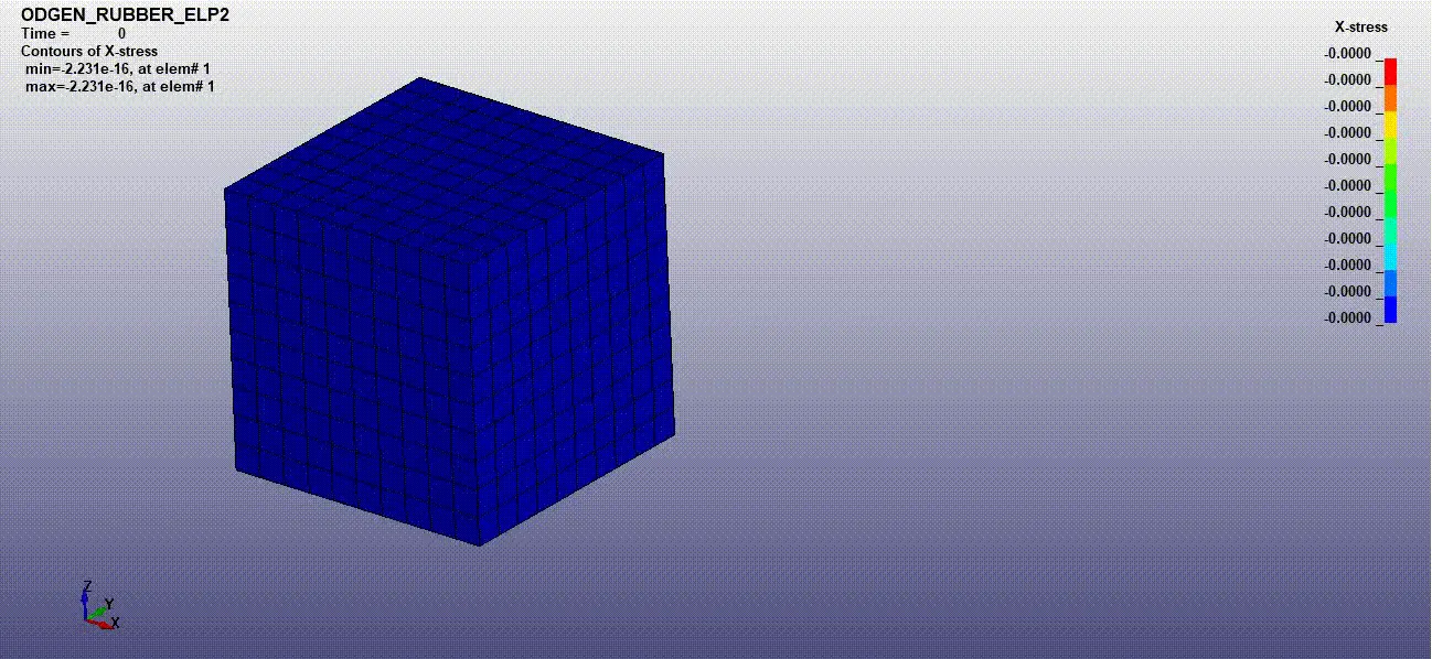
Fig, represents the X-STRESS ANIMATION of OGDEN MATERIAL with ELFORM 2

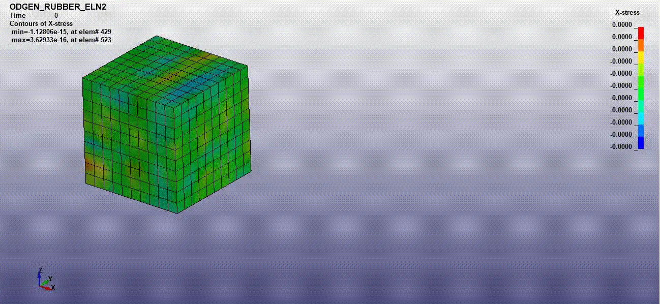
Fig, represents the X-STRESS ANIMATION of OGDEN MATERIAL with ELFORM -2

X-STRESS IMAGES OF ELFORM (1,-1,2,-2)

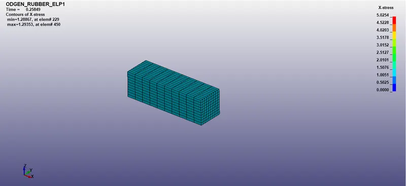
Fig (a), represents the X-STRESS Image of OGDEN MATERIAL with ELFORM 1

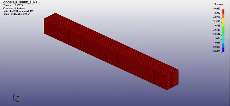
Fig(b), represents the X-STRESS Image of OGDEN MATERIAL with ELFORM -1

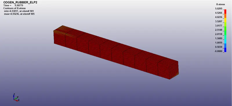
Fig (c), represents the X-STRESS Image of OGDEN MATERIAL with ELFORM 2

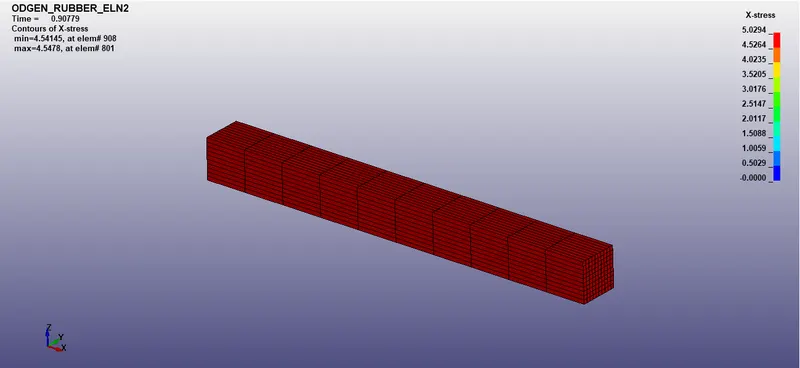
Fig(d), represents the X-STRESS Image of OGDEN MATERIAL with ELFORM -2

From, fig (a) & (b), it is observed that the Ogden material with ELFORM -1 has higher stress when compared to the ELFORM 1 but in both cases, there are only slight differences in their stress values.

From, fig (c) & (D), it is observed that the Ogden material with ELFORM 2 has higher stress when compared to the ELFORM -2 but in both cases, there are only slight differences in their stress values.

X-STRAIN IMAGES OF ELFORMS (1,-1,2,-2)

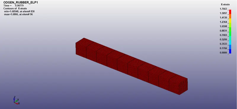
Fig(d), represents the X-STRAIN Image of OGDEN MATERIAL with ELFORM 1

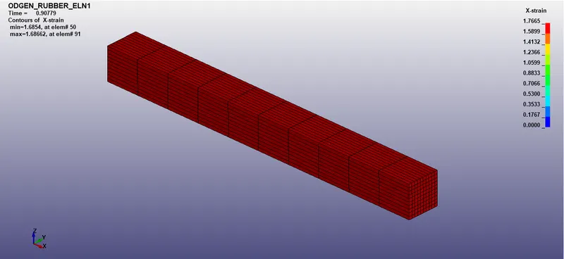
Fig(b), represents the X-STRAIN Image of OGDEN MATERIAL with ELFORM -1

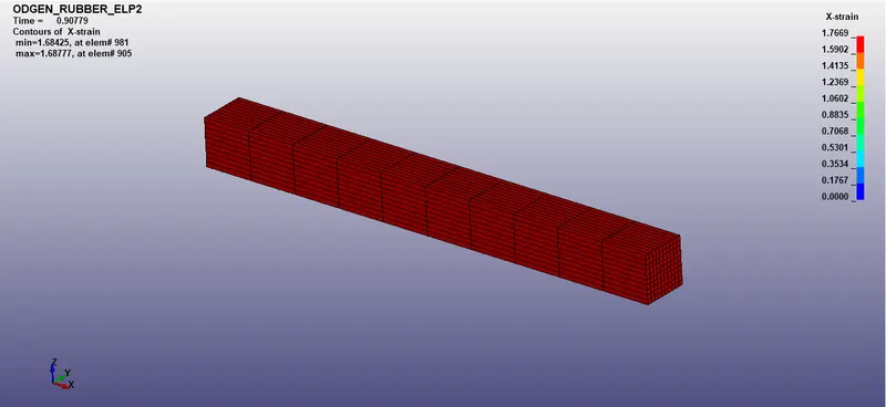
Fig(c), represents the X-STRAIN Image of OGDEN MATERIAL with ELFORM 2

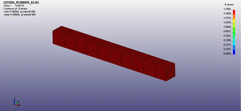
Fig(d), represents the X-STRAIN Image of OGDEN MATERIAL with ELFORM -2

From, fig (a) & (b), it is observed that the Ogden material with ELFORM -1 has a higher strain when compared to the ELFORM 1 but in both cases, there is an only a slight differences in their strain values.

From, fig (c) & (D), it is observed that the Ogden material with ELFORM 2 has higher strain when compared to the ELFORM -2 but in both cases, there is an only a slight difference in their strain values.

• The above stresses and strains that we obtained is called as True stress and true strains.
• By, knowing the true stress and strains we can calculate the engineering stress andengineering strain by the below formula.

FORMULAS USED TO CALCULATE ENGINEERING STRESS & STRAIN

Engineering stress, σe=σt/(1+ εe)= True stress / stretch ratio

True strain , εt=ln(1+ εe)

Engineering strain = εe=e^εt -1

Stretch ratio, Λ= 1+ εe

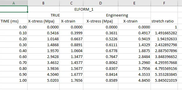
Fig, represents the calculation of engineering stress, engineering strain & stretch ratio for ELFORM 1

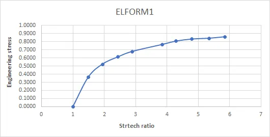
Fig, represents the engineering strain vs stretch ratio for ELFORM 1

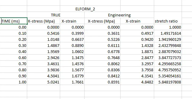
Fig, represents the calculation of engineering stress, engineering strain & stretch ratio for ELFORM 1

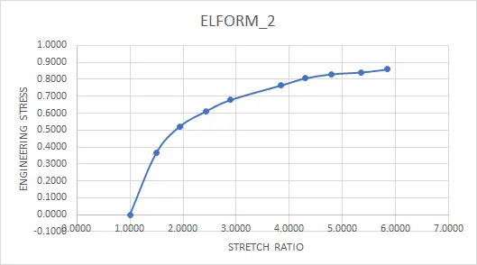
Fig, represents the engineering strain vs stretch ratio for ELFORM 2

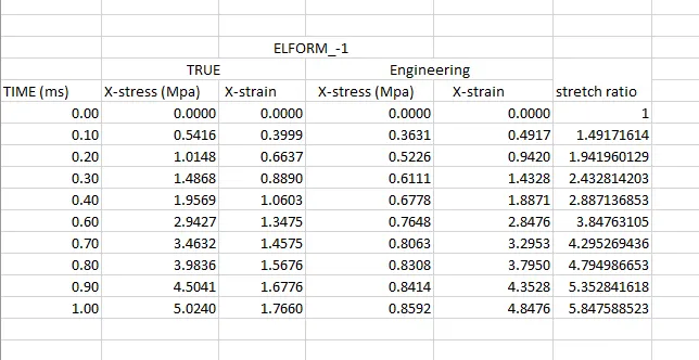
Fig, represents the calculation of engineering stress, engineering strain & stretch ratio for ELFORM -1

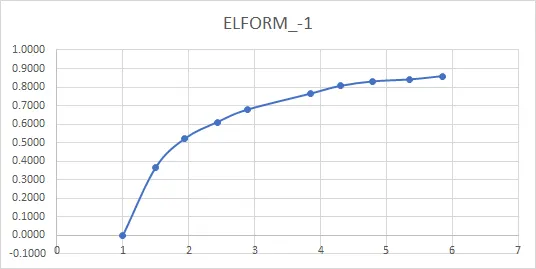
Fig, represents the engineering strain vs stretch ratio for ELFORM -1

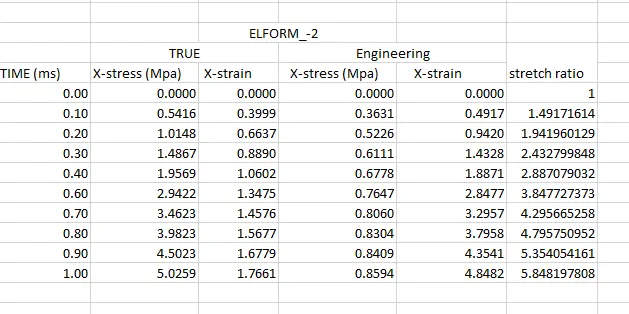
Fig, represents the calculation of engineering stress, engineering strain & stretch ratio for ELFORM -2

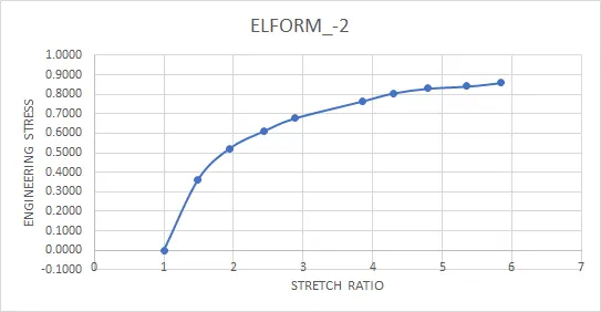
Fig, represents the engineering strain vs stretch ratio for ELFORM -2

• From, the above figures it is seen that the engineering stresses and stretch ratio's of various elform closely varies with one another but almost all their values are similar & but in reality the computational time for solving the iterations for different ELFORMS differs in solving the problem.

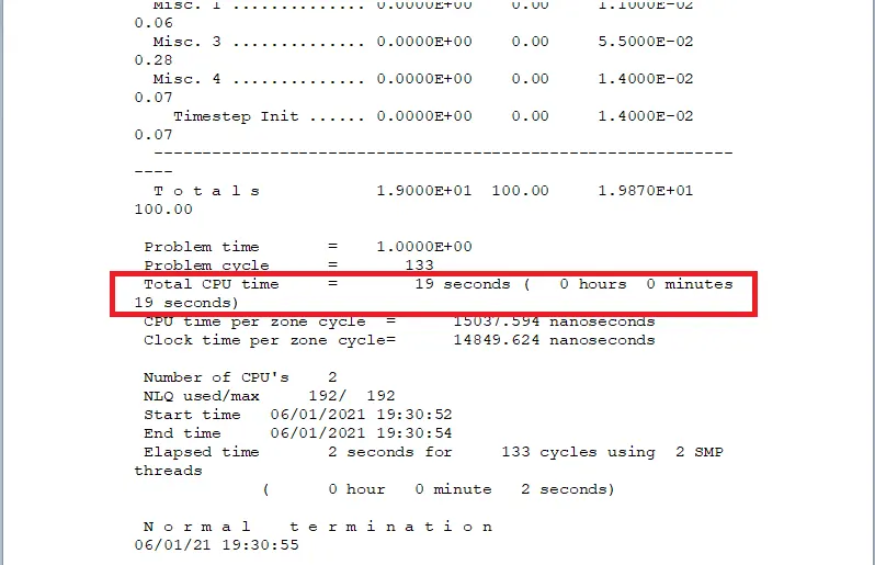
Fig, represents the computational time taken for solving the iterations for ELFORM 1

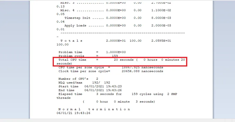
Fig, represents the computational time taken for solving the iterations for ELFORM -1

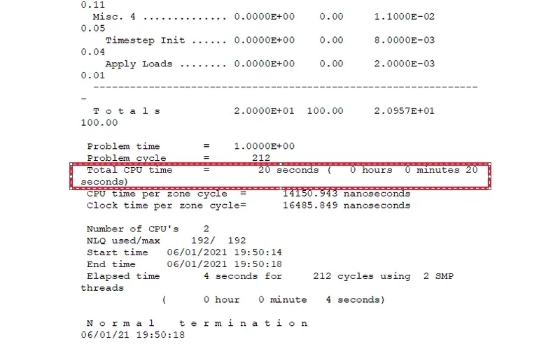
Fig, represents the computational time taken for solving the iterations for ELFORM 2

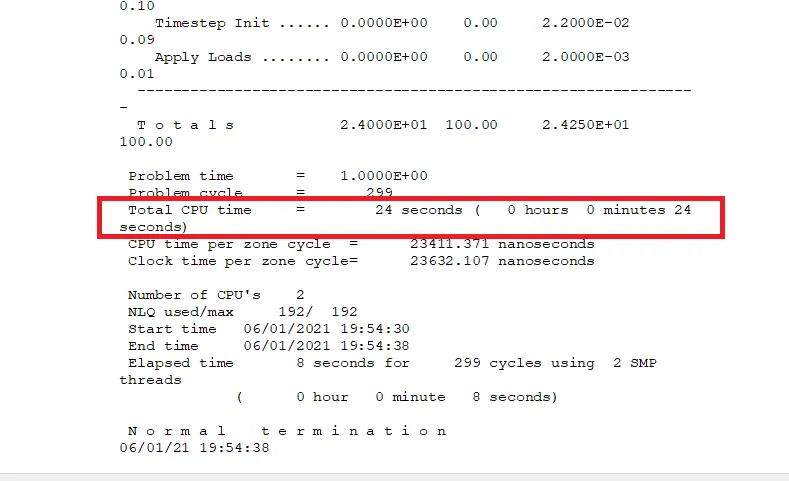
Fig, represents the computational time taken for solving the iterations for ELFORM -2

• The reason why the values are similar is the number of iterations slightly differ and the time for the computation for solving the problem is similar for different ELFORM (1,-1,2,-2)
• The values of the engineering stress vs stretch ratio slightly differ and they seem to be similar in the graphs.

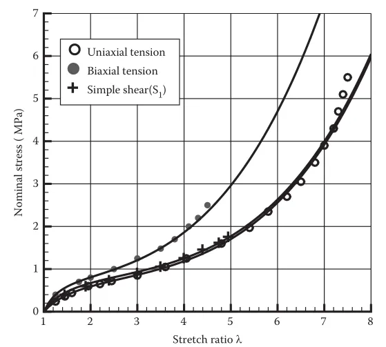
Fig, represents the Nominal stress Vs stretch ratio for the uniaxial plot.

• From, the graphs of various ELFORMS it is seen that the engineering stress VS stretch ratio is computed until stretch 5.84 for different ELFORMS and on the other hand in the uniaxial plot the engineering stress vs stretch ratio was computed till the stretch ratio 8.
• From, the graphs between ELFORMS VS UNIAXIAL PLOT it is clear that the stresses in the ELFORMS are computed to the 0.8 MPa and whereas in the uniaxial plot the stresses are plot till 7 Mpa.
• If we take the ranges of values from the ELFORMS and uniaxial plot to the stretch ratio of 5 it is clear that some values are slightly matches till the stretch ratio till 2 and they start to differ from the stretch ratio 3 indicating that there is a mismatch and this due to the different ELFORMS produces different types of engineering stress and stretch values.
• The reason why get such differences in the Uniaxial plot and ELFORMS plot is that the uniaxial plot has been tested with the actual material properties and here in the ELFORMS OF Ogden material the material properties are different from the actual testing and since the material properties such as Young's modulus changes we find that there is a difference in values and but the curve flows a similar fashion for the both plots.

CONCLUSION

• Thus, the input file for simulating the tensile test behavior is simulated successfully.
• The true stress, true strain, and engineering stresses and strains are calculated by using the required formulas.
• A proper excel sheet conversion is made for the different ELFORMS using (1,-1,2,-1) and different graphs are obtained for different ELFORMS.
• Finally, the graphs of different ELFORMS are compared against the uniaxial plot successfully