Week-6 Calculate the Stretch Ratio by comparing the ELFORM (-2,-1,1,2) with Ogden_Material Model.
OBJECTIVE
To carry out a tensile test on a created 10mmx10mmx10mm block and generate uniaxial tensile behavior results from simulation using either the explicit or implicit solver. Additionally, the results are compared between ELFORM 1, 2, -1 & -2 of the created block using a plot of Engineering Stress vs Stretch Ratio up to the stretch ratio 5. The material card to be used for this challenge is the ogden material, which has already been configured and provided.
BACKGROUND
The Ogden material model is a hyperelastic material model used to describe the non-linear stress-strain behavior of complex materials such as rubbers and biological tissue. The model was developed by Raymond Ogden in 1972. The model relies on the fact that the material behavior can be described by means of a strain energy density function, whence the stress-strain relationships can be derived. The Ogden model is often used to model rubberlike materials such as polymers, and biological materials. These materials can generally be considered to be isotropic, incompressible, and strain-rate independent.
In this challenge, we shall be comparing the results of 4 cases, differentiated by the type of element formulation used:
Case 1 - ELFORM 1: constant stress solid element.
Case 2 - ELFORM -1: Fully integrated S/R solid intended for elements with poor aspect ratio, efficient formulation.
Case 3 - ELFORM 2, Fully integrated S/R solid.
Case 4 - ELFORM -2, Fully integrated S/R solid intended for elements with poor aspect ratio, accurate formulation.
PROCEDURE
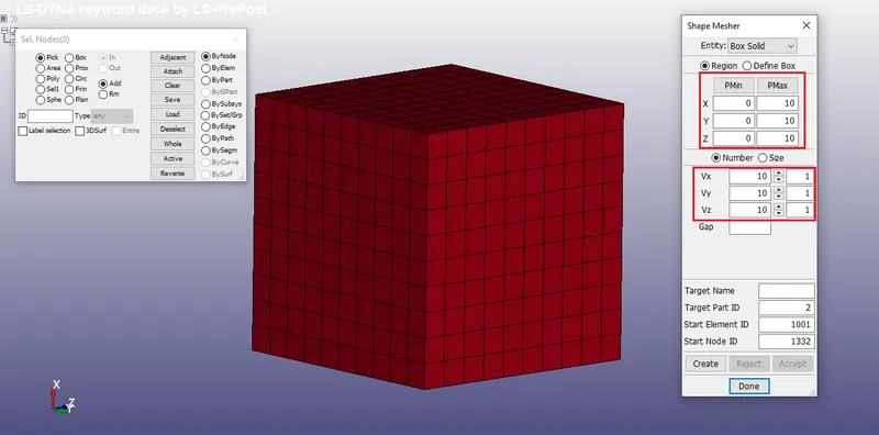
1. Firstly, on LS PrePost, the .k file containing the ogden material card is imported via File > Import > LS-DYNA keyword file. A solid block of 10mmx10mmx10mm dimension with 10 elements for each direction is created as shown:
2. The part contains solid elements and we are to assign a section card to it. So, we can access the keyword manager again, select the 'all' option, scroll to SECTION and select SOLID under it. We can assign a section ID with the ELFORM. This challenge requires us to compare the results of ELFORM 1, 2, -1, -2. So after simulation, this value is changed and the model is saved as a different file.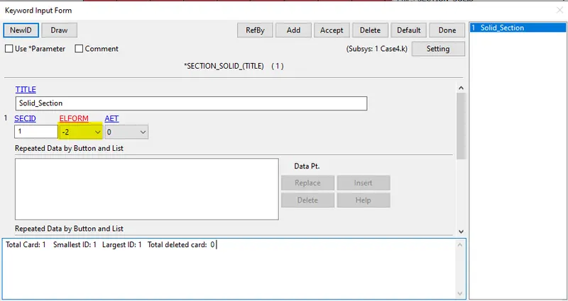
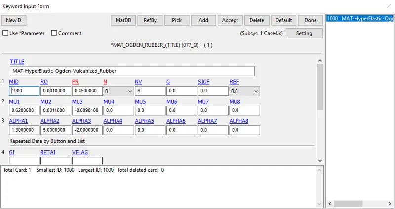
3. We can assign the MAT ID to the block we created as well. The material card for this does not require any editing. The following image shows the properties of the provided ogden material card:
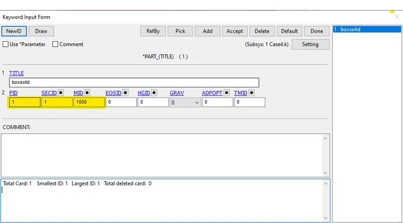
As mentioned previously, the MAT ID and SEC ID are applied to the block we just created:
4. There is no contact between parts or constituents within the simulation so we don't need to create a contact card for this model.
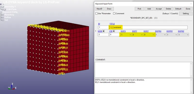
5. Moving on to the boundary conditions, we can assign the single point constraints on one side of the box. There are 3 separate SPCs we need to assign. Selecting all the nodes on that side, we can assign an SPC with an x-coordinate constraint only as shown:
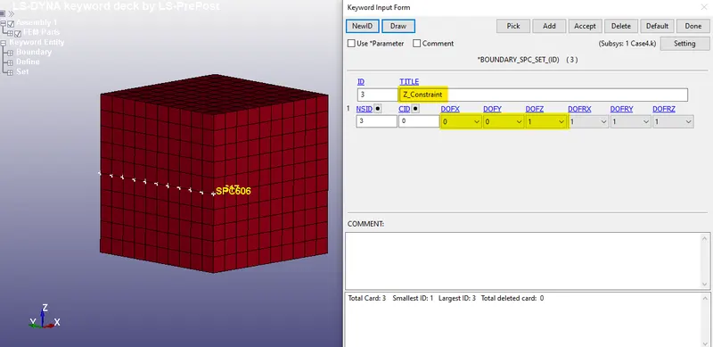
Then, selecting the nodes along the neutral axis (z direction) of the cube, we can constrain those nodes in the translational z coordinate as shown:
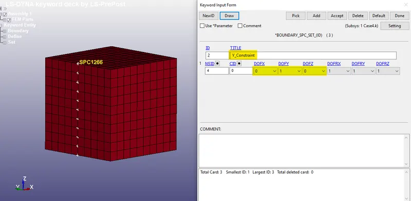
Similarly, the translational y coordinate is constrained for nodes along the neutral axis along y-direction as shown:
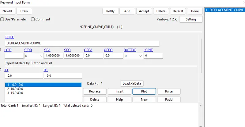
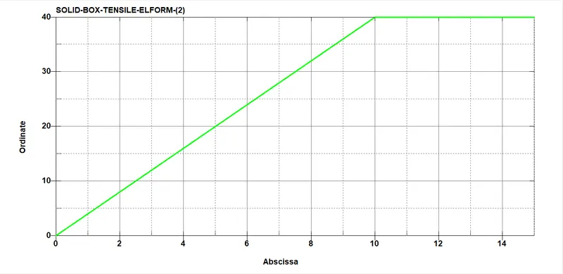
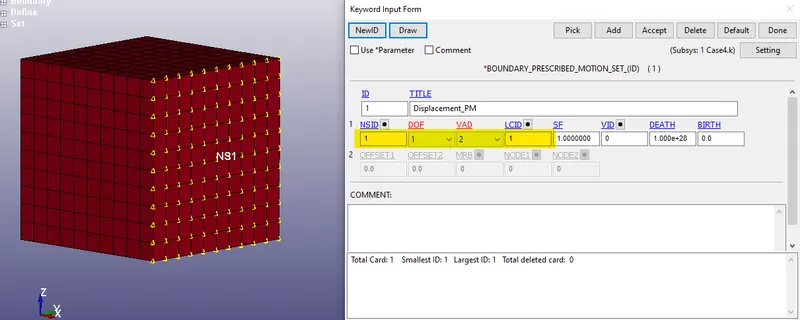
6. Next, we can assign the prescribed motion boundary condition to the opposite side of the box. We shall be utilizing the displacement variant of the condition. To define a BPM, a curve needs to be defined. We shall define one based on the stretch ratio mentioned for this challenge, which is 5. So the face is to be displaced by a minimum of 40mm.
Then, selecting all the nodes on the opposite face of the SPC nodes, the following card for prescribed motion was created:
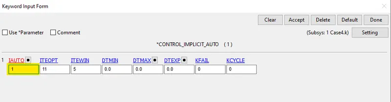
7. Implicit analysis is to be carried out on this model. To do that, some cards need to be activated - primarily *CONTROL_IMPLICIT_AUTO (for automatic time step control during implicit analysis) & *CONTROL_IMPLICIT_GENERAL (to initiate implicit analysis).
'1' for IMFLAG activates implicit analysis: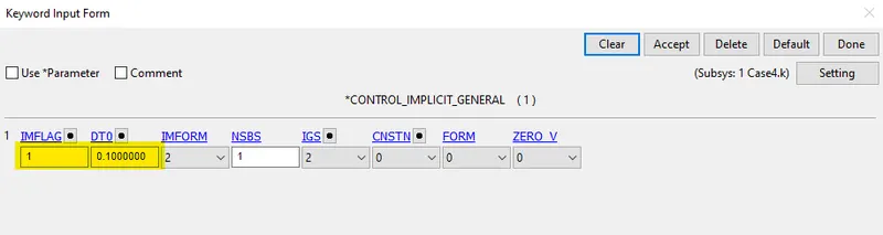
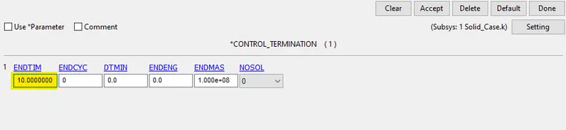
8. Next, we can create a CONTROL card to specify the end time of the simulation. This can be assigned via the TERMINATION card option under the CONTROL keyword in the complete list of keywords in the keyword manager. We can assign a value of 10ms to capture the entire simulation.
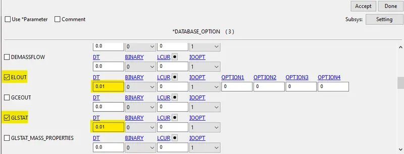
Finally, we can assign a couple of DATABASE keyword cards for the outputs - namely ASCII_option and BINARY_D3PLOT with a DT (Time interval between outputs) of 0.01ms. The GLSTAT, MATSUM & ELEOUT attributes are selected under ASCII_option.
The following screenshot shows the GLSTAT and ELOUT options selected. Energy values are written on a part-by-part basis in MATSUM and energy plots overall are evaluated using GLSTAT.
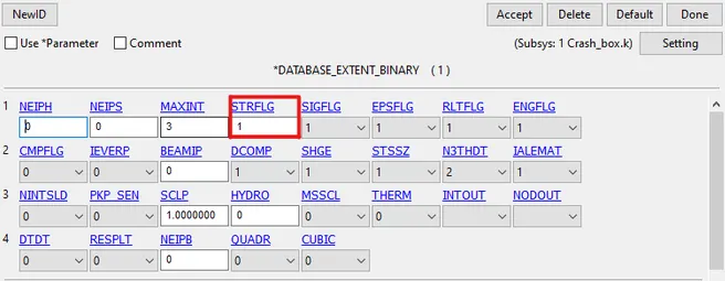
We also need to generate the strain outputs. To do that, we can create a keyword by going to Keyword manager and selecting DATABASE>EXTENT_BINARY. The DATABASE_EXTENT_BINARY card with STRFLG =1, would be used to compute the elastic strain in the model.
9. Once done, we can save it as a .k file and solve it using LS-RUN. The keyword file is inserted and we can click the play button to run the simulation. The number of cores to be utilised can be changed if needed.Once it is finished without errors (aka Normal Termination), we can reopen LS-Prepost to view the results. Again, the ELFORM value needs to be changed in the section card and the simulation repeated to reproduce the other three cases.
RESULTS
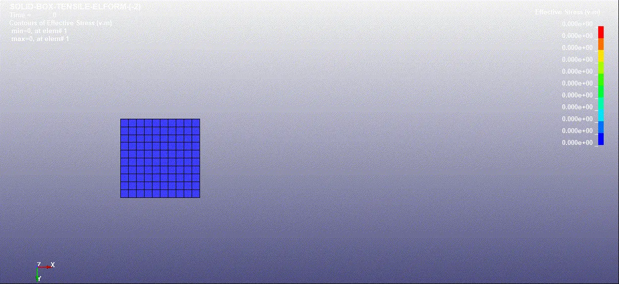
VON MISES STRESSES GENERATED
Case 1 (ELFORM 1)
Case 2 (ELFORM -1)
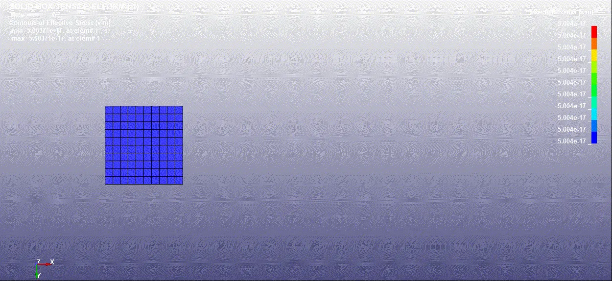
Case 3 (ELFORM 2)
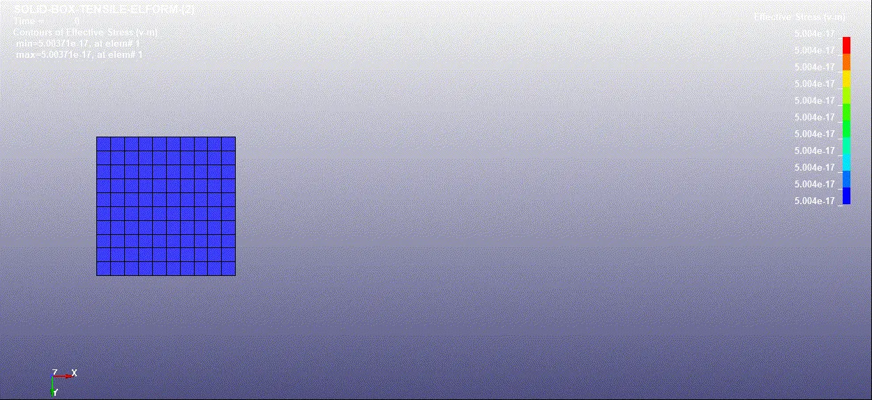
Case 4 (ELFORM -2)
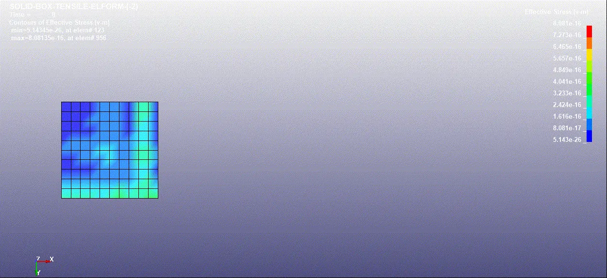
CALCULATION OF ENGINEERING STRESSES/STRAINS
In LS-DYNA the output of stress and strains is given as true stress and strains. To find the engineering stress/strain and stretch ratio, we need to make use of the following formulae:
We know that,
TRUE STRESS= ENG STRESS(1+ENG STRAIN)
TRUE STRAIN= ln (1+ ENG STRAIN)
From the simulation we got values for true stress and strain, so by using these values we can calculate the ENG STRESS AND STRAIN.
Let's calculate the ENG STRESS AND STRAIN FOR A time step-
From the simulation we have -
| Time(ms) | True_Stress_MPA | True_Strain |
| 0.00E+00 | 0.00E+00 | 0.00E+00 |
| 3.45E-01 | 1.60E-01 | 1.12E-02 |
by using the known formulas we got-
TRUE STRESS= ENG STRESS(1+ENG STRAIN)
0.16= ENG STRESS(1+ENG STRAIN).............(1)
We know that;
TRUE STRAIN=ln (1+ENG STRAIN)................(2)
ENG STRAIN= ln( 0.01120)-1
ENG STRAIN= 0.0113
Using this value in equation (1);
0.16= ENG STRESS(1+0.0113)
ENG STRESS=0.158 MPA
NOW WE HAVE ALL VALUES WE CAN CALCULATE THE STRETCH RATIO-
| Time(ms) | True_Stress_MPA | True_Strain | Nominal_stress_MPA | Nominal_strain |
| 0.00E+00 | 0.00E+00 | 0.00E+00 | 0.00E+00 | 0.00E+00 |
| 3.45E-01 | 1.60E-01 | 1.12E-02 | 1.58E-01 | 1.13E-02 |
| 6.90E-01 | 3.09E-01 | 3.92E-02 | 2.98E-01 | 3.99E-02 |
STRETCH RATIO,
λ=1+εe">λ=1+εe...........(3)
| Time(ms) | True_Stress_MPA | True_Strain | Nominal_stress_MPA | Nominal_strain | Strech_ratio(λ) |
| 0.00E+00 | 0.00E+00 | 0.00E+00 | 0.00E+00 | 0.00E+00 | 1.00E+00 |
| 3.45E-01 | 1.60E-01 | 1.12E-02 | 1.58E-01 | 1.13E-02 | 1.01E+00 |
Similarly, we can calculate the stress, strain, and stretch ratios for all values, all calculated results are given in the EXCEL SHEET FORMAT BELOW.
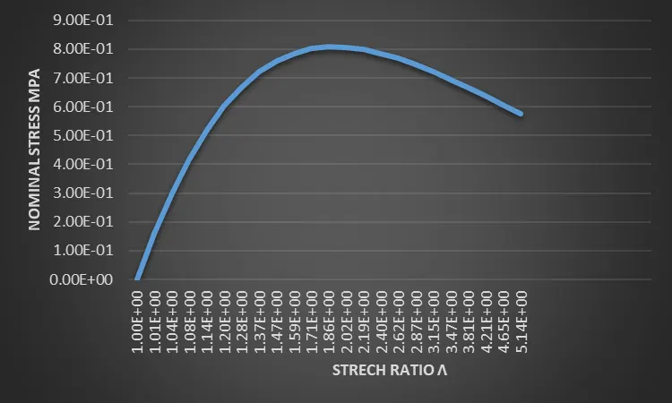
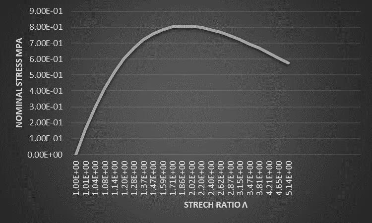
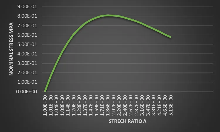
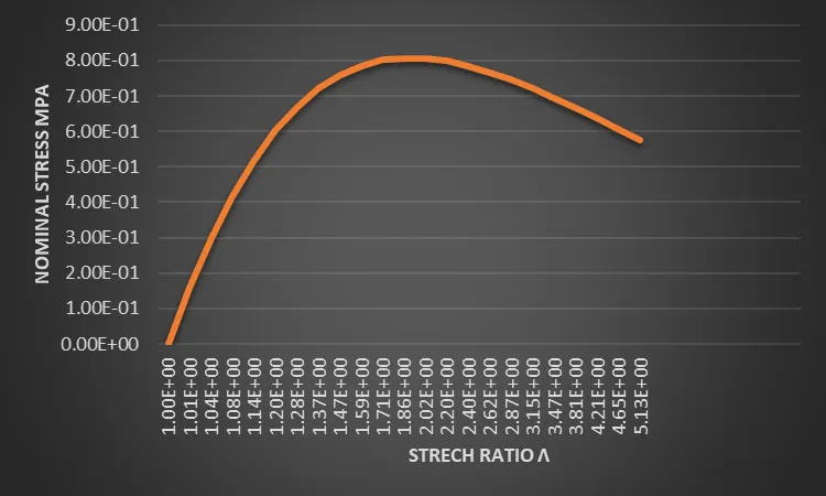
GRAPHS FOR ELFORM(1,2,-1,-2)-
1. ELFROM- 1:-
2. ELFORM-2:-
3. ELFORM-(-1):-
4.ELFORM-(-2):-
OBSERVATIONS
Looking at the plots of each case, we can see that the values obtained are pretty identical, only varying from the 4th or 5th decimal place or so. This also means that the engineering stress obtained for all cases when the stretch ratio is 5 is about 0.8 MPa. But taking a look at the original nominal stress vs stretch ratio plot provided:
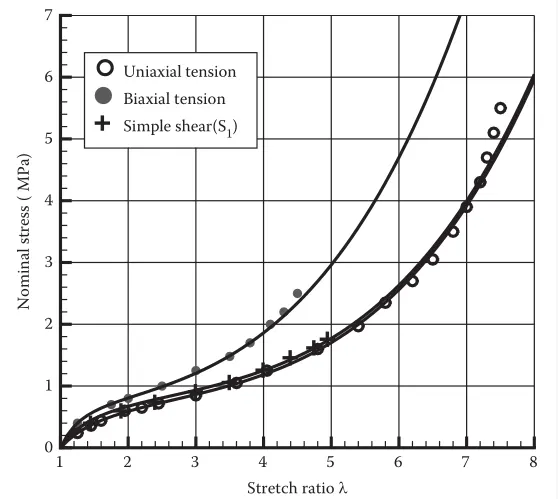
Ogden material is supposed to have a nominal stress value of 1.8MPa at a stretch ratio of 5. This could probably be due to the input of different material properties or boundary conditions. Furthermore, the simplicity of the simulation could also be a reason for this variation.
Finally, there is supposed to be a difference in computational time between each case but again, that is not discernable due to the simulation being very simple. But in more complex simulations, the reduced integrated element formulation (ELFORM 1) takes the least computational time followed by ELFORM 2. ELFORM -2 has a higher computational cost than ELFORM -1 and this is due to a difference in the formulation of the strain interpolation matrix.
CONCLUSION
A solid block FE element of specified dimensions was created and the provided Ogden material was applied to it, after which a uniaxial tensile test was carried out for four cases, each with different element formulations. The analysis was carried out with the help of the implicit solver in LS-Dyna, considering this test is considered quasi-static. The stretch ratio vs uniaxial engineering stress plots was created with the help of the results from the simulations.
LEARNING OUTCOME-
1. IN THIS CHALLENGE I LEARNED ABOUT THE THEORY BEHIND IMPLICIT ANALYSIS.
2. I LEARNED ABOUT THE EXECUTION OF IMPLICIT ANALYSIS.
3. LEARNED ABOUT DIFFERENT CONTROL_CARDS FOR INITIATING THE IMPLICIT ANALYSIS.
4. LEARNED HOW TO CHECK THE OUTPUT DATA AND HOW TO COMPARE IT WITH THE ANALYTICAL RESULTS.