Week 5 - Curve fitting

1. What do popt and pcov mean? (Watch the video to get some context)

Ans: popt : array Optimal values for the parameters so that the sum of the squared residuals of f (xdata, *popt) - ydata is minimized

pcov : 2d array The estimated covariance of popt. The diagonals provide the variance of the parameter estimate.

2. What does np.array(temperature) do?

Ans: numpy converts the list into a ndarray to perform mathematical functions.

3. What does the * in *popt mean?

Ans: *popt returns the coefficients stored in popt array calculated using curve_fit

4. Write code to fit a linear and cubic polynomial for the Cp data. Explain if your results are good or bad.

5. What needs to be done in order to make the curve fit perfect?

6. Show empirically how well your curve has been fit.

4,5,6 Ans:

Objective: To perform curve-fitting on given temperature and cp data using python.

Curve_fitting: is the process of constructing a curve, or mathematical function, that has the best fit to a series of data points, possibly subject to constraints. Curve fitting can involve either interpolation, where an exact fit to the data is required, or smoothing, in which a "smooth" function is constructed that approximately fits the data.

How do make a curve fit perfectly?

• A perfect Curve fit refers to that curve which mathematically represents the original data set, independent of the degree of a polynomial equation.
• A perfect Curve fit takes into consideration of most of the points in the data set, and the perfectness of the fit depends on the minimization of the error.

How to get the Best fit?

• the best fit Comes with no error/zero error after considering the values of the entire dataset
• The best fit line can be calculated by minimizing the distance between the actual and predicted output. There are several methods to do this like sum of squared errors, the sum of absolute errors, root mean squared error, etc.
• The difference between the predicted output and the actual output should be the least.

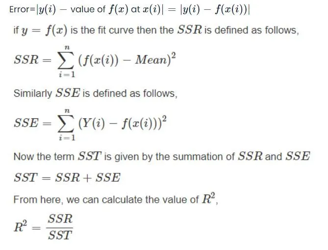
Governing Equations:

Code:

import numpy as np
import matplotlib.pyplot as plt
from scipy.optimize import curve_fit

#reading 'data' file and storing values in temperature and cp arrays
def read_file():
	temperature = []
	cp = []
	for line in open('data', 'r'):
		values = line.split(',')
		temperature.append(float(values[0]))
		cp.append(float(values[1]))
	return [temperature, cp]

#linear fit
def func_linear(t, a, b):
	return a*t +b

temperature, cp = read_file()
#calculating coefficients in the equation using curve_fit
popt, pocv = curve_fit(func_linear, temperature, cp)
#calculating cp using calculated coefficients
fit_cp_1 = func_linear(np.array(temperature), *popt)

#plotting linear equation
plt.figure('Linear')
plt.plot(temperature, cp, color = 'blue',linewidth = 4)
plt.plot(temperature, fit_cp_1, color = 'green')
plt.legend(['Actual data', 'Curve fit'])
plt.title('LINEAR CURVE FITTING')
plt.xlabel('Temperature [K]')
plt.ylabel('Cp')
plt.show()


#Quadratic curve fit
def func_quad(t, a, b, c):
	return a*pow(t,2) +b*t + c

temperature, cp = read_file()
#calculating coefficients in the equation using curve_fit
popt, pocv = curve_fit(func_quad, temperature, cp)
#calculating cp using calculated coefficients
fit_cp_2 = func_quad(np.array(temperature), *popt)

#plotting quadratic equation
plt.figure('Quadratic')
plt.plot(temperature, cp, color = 'blue', linewidth = 4 )
plt.plot(temperature, fit_cp_2, color = 'green')
plt.legend(['Actual data', 'Curve fit'])
plt.title('QUADRATIC CURVE FITTING')
plt.xlabel('Temperature [K]')
plt.ylabel('Cp')
plt.show()

#cubic curve fit
def func_cubic(t, a, b, c, d):
	return a*pow(t,3) +b*pow(t,2) + c*t + d

temperature, cp = read_file()
#calculating coefficients in the equation using curve_fit
popt, pocv = curve_fit(func_cubic, temperature, cp)
#calculating cp using calculated coefficients
fit_cp_3 = func_cubic(np.array(temperature), *popt)

#plotting cubic equation
plt.figure('Cubic')
plt.plot(temperature, cp, color = 'blue', linewidth = 4 )
plt.plot(temperature, fit_cp_3, color = 'green')
plt.legend(['Actual data', 'Curve fit'])
plt.title('CUBIC CURVE FITTING')
plt.xlabel('Temperature [K]')
plt.ylabel('Cp')
plt.show()




# bi-quadratic curve fit
def func_biQ(t, a, b, c, d, e):
	return a*pow(t,4) +b*pow(t,3) + c*pow(t,2) + d*t + e

temperature, cp = read_file()
#calculating coefficients in the equation using curve_fit
popt, pocv = curve_fit(func_biQ, temperature, cp)
#calculating cp using calculated coefficients
fit_cp_4 = func_biQ(np.array(temperature), *popt)

#plotting bi-quadratic equation
plt.figure('BIQUADRATIC')
plt.plot(temperature, cp, color = 'blue', linewidth = 4  )
plt.plot(temperature, fit_cp_4, color = 'green')
plt.legend(['Actual data', 'Curve fit'])
plt.title('BIQUADRATIC CURVE FITTING')
plt.xlabel('Temperature [K]')
plt.ylabel('Cp')
plt.show()

#higher polynomial curve fit
def func_7D(t, a, b, c, d, e, f,g,h):
	return a*pow(t,7) +b*pow(t,6) + c*pow(t,5) + d*pow(t,4) + e*pow(t,3) + f*pow(t,2) +g*t +h

temperature, cp = read_file()
#calculating coefficients in the equation using curve_fit
popt, pocv = curve_fit(func_7D, temperature, cp)
#calculating cp using calculated coefficients
fit_cp_7 = func_7D(np.array(temperature), *popt)

#plotting bi-quadratic equation
plt.figure('7th Degree Polynomial')
plt.plot(temperature, cp, color = 'blue', linewidth = 4 )
plt.plot(temperature, fit_cp_7, color = 'green')
plt.legend(['Actual data', 'Curve fit'])
plt.title('Higher Polynomial')
plt.xlabel('Temperature [K]')
plt.ylabel('Cp')
plt.show()


# Fitness Characteristics Calculation
sum1 = np.sum(cp)
n = np.size(cp)

# Mean
mean = sum1/n

# For Linear Curve Fit
SSR_lin = 0
SSE_lin = 0

for i in range(n):
	error = abs((np.sum((cp[i] - fit_cp_1[i]))))
	SSE_lin = SSE_lin + pow(error,2)
	SSR_lin = SSR_lin + (np.sum(pow((fit_cp_1[i] - mean),2)))

SST_lin = SSE_lin + SSR_lin
Rsq_lin = SSR_lin/SST_lin
RMSE_lin = pow((SSE_lin/n),0.5)

print('Linear curve_fit characteristics')
print('SST_lin:', SST_lin)
print('Rsq_lin:', Rsq_lin)
print('RMSE_lin:', RMSE_lin)
print('----------------------------------')
# For Quadratic Curve Fit
SSR_quad = 0
SSE_quad = 0

for i in range(n):
	error = abs((np.sum((cp[i] - fit_cp_2[i]))))
	SSE_quad = SSE_quad + pow(error,2)
	SSR_quad = SSR_quad + (np.sum(pow((fit_cp_2[i] - mean),2)))

SST_quad = SSE_quad + SSR_quad
Rsq_quad = SSR_quad/SST_quad
RMSE_quad = pow((SSE_quad/n),0.5)
print('Quadratic curve_fit characteristics')
print('SST_quad:', SST_quad)
print('Rsq_quad:', Rsq_quad)
print('RMSE_quad:', RMSE_quad)
print('----------------------------------')

# For Cubic Curve Fit
SSR_cub = 0
SSE_cub = 0

for i in range(n):
	error = abs((np.sum((cp[i] - fit_cp_3[i]))))
	SSE_cub = SSE_cub + pow(error,2)
	SSR_cub = SSR_cub + (np.sum(pow((fit_cp_3[i] - mean),2)))

SST_cub = SSE_cub + SSR_cub
Rsq_cub = SSR_cub/SST_cub
RMSE_cub = pow((SSE_cub/n),0.5)

print('Cubic curve_fit characteristics')
print('SST_cub:', SST_cub)
print('Rsq_cub:', Rsq_cub)
print('RMSE_cub:', RMSE_cub)
print('----------------------------------')

# For Biquadratic Curve Fit
SSR_bquad = 0
SSE_bquad = 0

for i in range(n):
	error = abs((np.sum((cp[i] - fit_cp_4[i]))))
	SSE_bquad = SSE_bquad + pow(error,2)
	SSR_bquad = SSR_bquad + (np.sum(pow((fit_cp_4[i] - mean),2)))

SST_bquad = SSE_bquad + SSR_bquad
Rsq_bquad = SSR_bquad/SST_bquad
RMSE_bquad = pow((SSE_bquad/n),0.5)

print('Biquadratic curve_fit characteristics')
print('SST_bquad:', SST_bquad)
print('Rsq_bquad:', Rsq_bquad)
print('RMSE_bquad:', RMSE_bquad)
print('----------------------------------')

#For higher polynomial fit
SSR_bquad = 0
SSE_bquad = 0

for i in range(n):
	error = abs((np.sum((cp[i] - fit_cp_7[i]))))
	SSE_bquad = SSE_bquad + pow(error,2)
	SSR_bquad = SSR_bquad + (np.sum(pow((fit_cp_7[i] - mean),2)))

SST_bquad = SSE_bquad + SSR_bquad
Rsq_bquad = SSR_bquad/SST_bquad
RMSE_bquad = pow((SSE_bquad/n),0.5)

print('Higher Polynomial curve_fit characteristics')
print('SST_bquad:', SST_bquad)
print('Rsq_bquad:', Rsq_bquad)
print('RMSE_bquad:', RMSE_bquad)
print('----------------------------------')

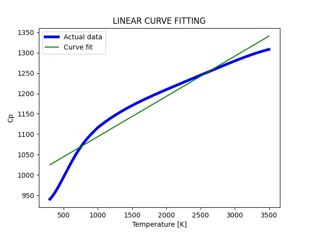
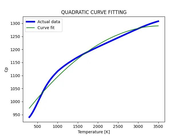
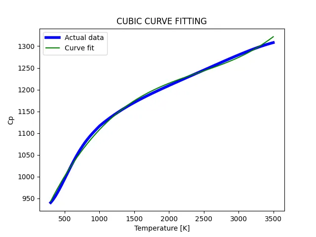
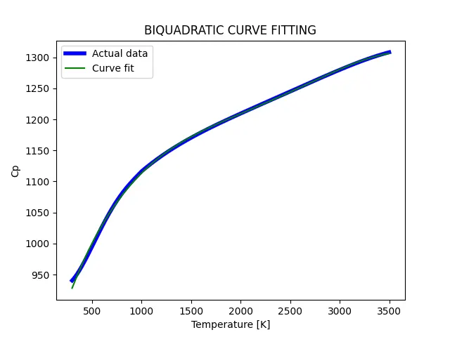
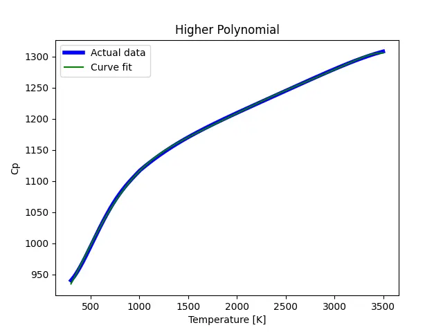
The above code calculates the coefficients for linear, quadratic, cubic, bi-quadratic and 7th-degree polynomial relation between cp and temperature and re-calculates cp as fit_cp using coefficients from popt and temperature from data.

Accordingly graphs were plotted, cp vs temperature from data and fit_cp vs temperature.

The graphs are as follows:

Conclusion:

After observing above graphs, linear and quadratic curves are not the best fit for the actual data curve.

Cubic curve provides the better fit but not as smooth as bi-quadratic. As the degree of polynomial was raised the curve is getting better smooth and R-square is too getting closer to 1 as expected but this provides the multiple answers and doesn't't end up with where to stop the fit. In such case the lower the degree of polynomial with better smooth. In this case, Bi-quadratic equation gives better fit.