Project 12

Conditional GAN (cGAN)
Generative Adversarial Network

Abstract
Generative Adversarial Networks, or GANs, are an architecture for training generative models, such as deep convolutional neural networks for generating images. Here in this project, a conditional GAN is applied to generate and train a model to generate images of aeroplanes, automobiles, birds, cats, deer, frogs, horses, ships and trucks based on the classes and dataset of CIFAR10.

Introduction
Although GAN models are capable of generating new random plausible examples for a given dataset, there is no way to control the types of images that are generated other than trying to figure out the complex relationship between the latent space input to the generator and the generated images.
The conditional generative adversarial network, or cGAN for short, is a type of GAN that involves the conditional generation of images by a generator model. Image generation can be conditional on a class label, if available, allowing the targeted generated of images of a given type.
The architecture is comprised of a generator and a discriminator model. The generator model is responsible for generating new plausible examples that ideally are indistinguishable from real examples in the dataset. The discriminator model is responsible for classifying a given image as either real (drawn from the dataset) or fake (generated).
The models are trained together in a zero-sum or adversarial manner, such that improvements in the discriminator come at the cost of a reduced capability of the generator, and vice versa.
GANs are effective at image synthesis, that is, generating new examples of images for a target dataset. Some datasets have additional information, such as a class label, and it is desirable to make use of this information.
The CIFAR-10 small object photograph dataset has class labels for the corresponding objects in the photographs.
The Fashion-MNIST clothing dataset has class labels for the corresponding items of clothing.
There are two motivations for making use of the class label information in a GAN model.
Improve the GAN.
Targeted Image Generation.

Class labels can also be used for the deliberate or targeted generation of images of a given type. For example, in the case of CIFAR-10, specific object photographs can be generated such as ‘frogs‘.

CIFAR10 Dataset:
The CIFAR-10 dataset consists of 60000 32x32 colour images in 10 classes, with 6000 images per class. There are 50000 training images and 10000 test images.

The dataset is divided into five training batches and one test batch, each with 10000 images. The test batch contains exactly 1000 randomly-selected images from each class. The training batches contain the remaining images in random order, but some training batches may contain more images from one class than another. Between them, the training batches contain exactly 5000 images from each class.

The classes of Dataset are:
0. Airplane
1. Automobile
2. Bird
3. Cat
4. Deer
5. Dog
6. Frog
7. Horse
8. Ship
9. Truck

CODE

Import all the necessary modules numpy, keras, keras layers, optimizers and cifar10 dataset.

from numpy import zeros
from numpy import ones
from numpy.random import randn
from numpy.random import randint
from keras.datasets.cifar10 import load_data
from keras.optimizers import Adam
from keras.models import Model
from keras.layers import Input
from keras.layers import Dense
from keras.layers import Reshape
from keras.layers import Flatten
from keras.layers import Conv2D
from keras.layers import Conv2DTranspose
from keras.layers import LeakyReLU
from keras.layers import Dropout
from keras.layers import Embedding
from keras.layers import Concatenate
import os
import sys 
from matplotlib import pyplot as plt

Loading a small sample from CIFAR dataset.
This downloads data from cs.toronto.edu and displays some photographs of the dataset.

#Load data and plot to get a quick understanding
#CIFAR10 classes are: airplane, automobile, bird, cat, deer, dog, frog, horse,
# ship, truck

(trainX, trainy), (testX, testy) = load_data()

# plot 25 images
for i in range(25):
	plt.subplot(5, 5, 1 + i)
	plt.axis('off')
	plt.imshow(trainX[i])
plt.show()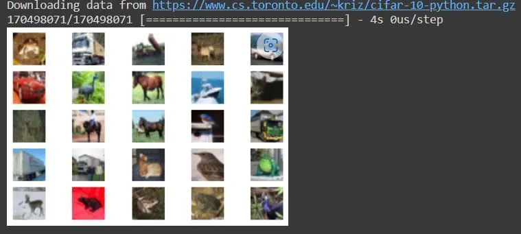

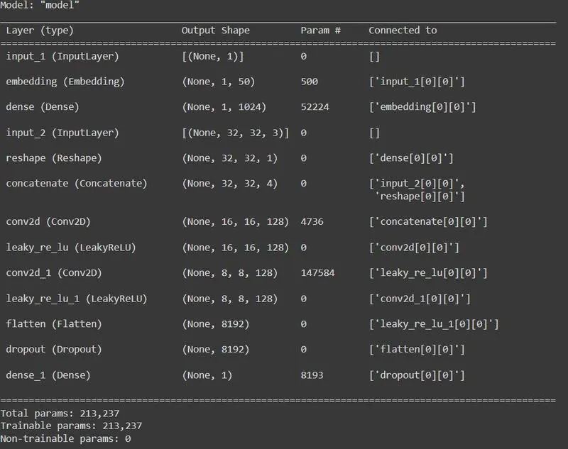
Defining the discriminator model.
Given an input image, the discriminator outputs the likelihood of the image is real (0 or 1). Binary classification, so sigmoid activation is used here.

def define_discriminator(in_shape=(32,32,3), n_classes=10):
	
    # label input
	in_label = Input(shape=(1,))  #Shape 1
	# embedding for categorical input
    #each label (total 10 classes for cifar), will be represented by a vector of size 50. 
    #This vector of size 50 will be learnt by the discriminator
	li = Embedding(n_classes, 50)(in_label) #Shape 1,50
	# scale up to image dimensions with linear activation
	n_nodes = in_shape[0] * in_shape[1]  #32x32 = 1024. 
	li = Dense(n_nodes)(li)  #Shape = 1, 1024
	# reshape to additional channel
	li = Reshape((in_shape[0], in_shape[1], 1))(li)  #32x32x1
    
    
	# image input
	in_image = Input(shape=in_shape) #32x32x3
	# concat label as a channel
	merge = Concatenate()([in_image, li]) #32x32x4 (4 channels, 3 for image and the other for labels)
    
	# downsample: This part is same as unconditional GAN upto the output layer.
    #We will combine input label with input image and supply as inputs to the model. 
	fe = Conv2D(128, (3,3), strides=(2,2), padding='same')(merge) #16x16x128
	fe = LeakyReLU(alpha=0.2)(fe)
	# downsample
	fe = Conv2D(128, (3,3), strides=(2,2), padding='same')(fe) #8x8x128
	fe = LeakyReLU(alpha=0.2)(fe)
	# flatten feature maps
	fe = Flatten()(fe)  #8192  (8*8*128=8192)
	# dropout
	fe = Dropout(0.4)(fe)
	# output
	out_layer = Dense(1, activation='sigmoid')(fe)  #Shape=1
    
	# define model
    ##Combine input label with input image and supply as inputs to the model. 
	model = Model([in_image, in_label], out_layer)
	# compile model
	opt = Adam(learning_rate=0.0002, beta_1=0.5)
	model.compile(loss='binary_crossentropy', optimizer=opt, metrics=['accuracy'])
	return model

printing its summary

test_discr = define_discriminator()

print(test_discr.summary())

Defining the generator model
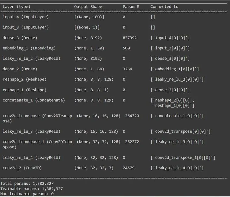
Latent vectors and labels are given as inputs with classes

def define_generator(latent_dim, n_classes=10):
    
	# label input
	in_label = Input(shape=(1,))  #Input of dimension 1
	# embedding for categorical input
    #each label (total 10 classes for cifar), will be represented by a vector of size 50. 
	li = Embedding(n_classes, 50)(in_label) #Shape 1,50
    
	# linear multiplication
	n_nodes = 8 * 8  # To match the dimensions for concatenation later in this step.  
	li = Dense(n_nodes)(li) #1,64
	# reshape to additional channel
	li = Reshape((8, 8, 1))(li)
    
    
	# image generator input
	in_lat = Input(shape=(latent_dim,))  #Input of dimension 100
    
	# foundation for 8x8 image
    # We will reshape input latent vector into 8x8 image as a starting point. 
    #So n_nodes for the Dense layer can be 128x8x8 so when we reshape the output 
    #it would be 8x8x128 and that can be slowly upscaled to 32x32 image for output.
    #Note that this part is same as unconditional GAN until the output layer. 
    #While defining model inputs we will combine input label and the latent input.
	n_nodes = 128 * 8 * 8
	gen = Dense(n_nodes)(in_lat)  #shape=8192
	gen = LeakyReLU(alpha=0.2)(gen)
	gen = Reshape((8, 8, 128))(gen) #Shape=8x8x128
	# merge image gen and label input
	merge = Concatenate()([gen, li])  #Shape=8x8x129 (Extra channel corresponds to the label)
	# upsample to 16x16
	gen = Conv2DTranspose(128, (4,4), strides=(2,2), padding='same')(merge) #16x16x128
	gen = LeakyReLU(alpha=0.2)(gen)
	# upsample to 32x32
	gen = Conv2DTranspose(128, (4,4), strides=(2,2), padding='same')(gen) #32x32x128
	gen = LeakyReLU(alpha=0.2)(gen)
	# output
	out_layer = Conv2D(3, (8,8), activation='tanh', padding='same')(gen) #32x32x3
	# define model
	model = Model([in_lat, in_label], out_layer)
	return model

Printing summary of generator model

test_gen = define_generator(100, n_classes=10)

print(test_gen.summary())

Generator is trained via GAN combined model but discriminator.
Define the combined generator and discriminator model for updating the generator.
But Discriminator is trained independently so for now only generator is the only one being trained with discriminator being constant

def define_gan(g_model, d_model):
	d_model.trainable = False  #Discriminator is trained separately. So set to not trainable.
    
    ## connect generator and discriminator...
	# first, get noise and label inputs from generator model
	gen_noise, gen_label = g_model.input  #Latent vector size and label size
	# get image output from the generator model
	gen_output = g_model.output  #32x32x3
    
	# generator image output and corresponding input label are inputs to discriminator
	gan_output = d_model([gen_output, gen_label])
	# define gan model as taking noise and label and outputting a classification
	model = Model([gen_noise, gen_label], gan_output)
	# compile model
	opt = Adam(lr=0.0002, beta_1=0.5)
	model.compile(loss='binary_crossentropy', optimizer=opt)
	return model

Loading cifar images

def load_real_samples():
	# load dataset
	(trainX, trainy), (_, _) = load_data()   #cifar
	# convert to floats and scale
	X = trainX.astype('float32')
	# scale from [0,255] to [-1,1]
	X = (X - 127.5) / 127.5   
                           
	return [X, trainy]

Now train the GAN on a half batch of real images and another half batch of fake images
For each real image we assign a label 1 and for fake label 0

def generate_real_samples(dataset, n_samples):
	# split into images and labels
	images, labels = dataset  
	# choose random instances
	ix = randint(0, images.shape[0], n_samples)
	# select images and labels
	X, labels = images[ix], labels[ix]
	# generate class labels and assign to y
	y = ones((n_samples, 1))  #Label=1 indicating they are real
	return [X, labels], y

Generating points in latent space as input for the generator

def generate_latent_points(latent_dim, n_samples, n_classes=10):
	# generate points in the latent space
	x_input = randn(latent_dim * n_samples)
	# reshape into a batch of inputs for the network
	z_input = x_input.reshape(n_samples, latent_dim)
	# generate labels
	labels = randint(0, n_classes, n_samples)
	return [z_input, labels]

Here fake images are predicted using the generator model with class labels with latent dimensions

def generate_fake_samples(generator, latent_dim, n_samples):
	# generate points in latent space
	z_input, labels_input = generate_latent_points(latent_dim, n_samples)
	# predict outputs
	images = generator.predict([z_input, labels_input])
	# create class labels
	y = zeros((n_samples, 1))  #Label=0 indicating they are fake
	return [images, labels_input], y

Train the generator and discriminator by looping through number of epochs to train discriminator with a random batch of images from dataset (real)
Then set of images are generated using the generator
Feed the discriminator with both set of images
And set the loss parameters for both real and fake images and the combined loss

def train(g_model, d_model, gan_model, dataset, latent_dim, n_epochs=100, n_batch=128):
	bat_per_epo = int(dataset[0].shape[0] / n_batch)
	half_batch = int(n_batch / 2)  #the discriminator model is updated for a half batch of real samples 
                            #and a half batch of fake samples, combined a single batch. 
	# manually enumerate epochs
	for i in range(n_epochs):
		# enumerate batches over the training set
		for j in range(bat_per_epo):
			
             # Train the discriminator on real and fake images, separately (half batch each)
        #Research showed that separate training is more effective. 
			# get randomly selected 'real' samples
            # get randomly selected 'real' samples
			[X_real, labels_real], y_real = generate_real_samples(dataset, half_batch)

            # update discriminator model weights
            ##train_on_batch allows you to update weights based on a collection 
            #of samples you provide
			d_loss_real, _ = d_model.train_on_batch([X_real, labels_real], y_real)
            
			# generate 'fake' examples
			[X_fake, labels], y_fake = generate_fake_samples(g_model, latent_dim, half_batch)
			# update discriminator model weights
			d_loss_fake, _ = d_model.train_on_batch([X_fake, labels], y_fake)
            
            #d_loss = 0.5 * np.add(d_loss_real, d_loss_fake) #Average loss if you want to report single..
            
			# prepare points in latent space as input for the generator
			[z_input, labels_input] = generate_latent_points(latent_dim, n_batch)
            
            # The generator wants the discriminator to label the generated samples
        # as valid (ones)
        #This is where the generator is trying to trick discriminator into believing
        #the generated image is true (hence value of 1 for y)	
			# create inverted labels for the fake samples
			y_gan = ones((n_batch, 1))
             # Generator is part of combined model where it got directly linked with the discriminator
        # Train the generator with latent_dim as x and 1 as y. 
        # Again, 1 as the output as it is adversarial and if generator did a great
        #job of folling the discriminator then the output would be 1 (true)
			# update the generator via the discriminator's error
			g_loss = gan_model.train_on_batch([z_input, labels_input], y_gan)
			# Print losses on this batch
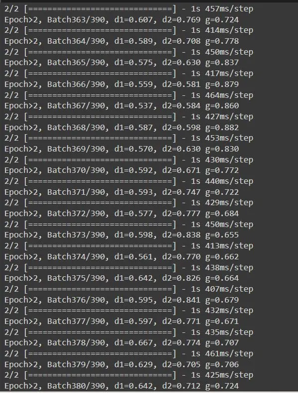
			print('Epoch>%d, Batch%d/%d, d1=%.3f, d2=%.3f g=%.3f' %
				(i+1, j+1, bat_per_epo, d_loss_real, d_loss_fake, g_loss))
	# save the generator model
	g_model.save('/content/cifar_conditional_generator_25epochs.h5')

Train the gan and create the cifar train model

# size of the latent space
latent_dim = 100
# create the discriminator
d_model = define_discriminator()
# create the generator
g_model = define_generator(latent_dim)
# create the gan
gan_model = define_gan(g_model, d_model)
# load image data
dataset = load_real_samples()
# train model
train(g_model, d_model, gan_model, dataset, latent_dim, n_epochs=2)

Output:

Lastly plot results based on the trained model h5 file

from numpy import asarray
from numpy.random import randn
from numpy.random import randint
from keras.models import load_model
import numpy as np
# 
import sys
import os


#Note: CIFAR10 classes are: airplane, automobile, bird, cat, deer, dog, frog, horse,
# ship, truck

# load model
model = load_model('/contents/cifar_conditional_generator_25epochs.h5')

# generate multiple images

latent_points, labels = generate_latent_points(100, 100)
# specify labels - generate 10 sets of labels each gping from 0 to 9
labels = asarray([x for _ in range(10) for x in range(10)])
# generate images
X  = model.predict([latent_points, labels])
# scale from [-1,1] to [0,1]
X = (X + 1) / 2.0
X = (X*255).astype(np.uint8)
# plot the result (10 sets of images, all images in a column should be of same class in the plot)
# Plot generated images 
def show_plot(examples, n):
	for i in range(n * n):
		plt.subplot(n, n, 1 + i)
		plt.axis('off')
		plt.imshow(examples[i, :, :, :])
	plt.show()
    
show_plot(X, 10)

The results are as follows

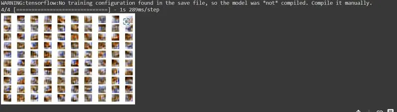
The results are after running the train for just 2 epochs, which took 2.5 hrs to train on google colabs and colabs refreshes after every 90 mins of inactivity, which made me stop at 2 epochs. As the training increases the images get better.