Curve fitting using Python

OBJECTIVE:

To perform curve fitting using python for the given Cp vs Temperature data file.

THEORY:

Curve fitting is the process of constructing a curve, or mathematical function, that has the best fit to a series of data points, possibly subject to constraints. It can involve either interpolation, where an exact fit to the data is required or smoothing, in which a "smooth" function is constructed that approximately fits the data.

SOLUTION:

1. What does popt and pcov mean?

Ans: "popt" - It is an array which stores the optimal value of coefficients that are being passed in a given function so that the sum of squared residuals of is f(xdata, *popt) - ydata minimised.

"pcov" - It is a two dimensional array that stores the estimated values of the estimated covariance of popt. The diagonals of the array provide the variance of the parameter estimate. The function perr = np.sqrt(np.diag(pcov)) is used to compute one standard deviation on the parameters.

2. What does np.array(temperature) do?

Ans: NumPy is a general purpose array-processing package. np.array(temperature) is used for passing the values of temperature as a numpy array.

3. What does the * in *popt mean?

Ans: The * notation will expand a list of values into the arguments of a function. It is useful if the function has more than one or two parameters. Here, * refers to the coefficients in a given equation.

4. Write code to fit a linear and cubic polynomial for the Cp data. Explain if your results are good or bad.

#Curve fitting by Ashwen Venkatesh
import numpy as np 
import matplotlib.pyplot as plt 
from scipy.optimize import curve_fit

#Function for cubic curve fit
def func_cubic(t,a,b,c,d):
	return a*pow(t,3) + b*pow(t,2) + c*t + d

#Function for linear curve fit
def func_linear(t,a,b):
	return a*t + b

#Function for reding the contents of data file
def read_file():
	temperature=[]
	cp=[]
	for line in open('data','r'):
		values= line.split(',')
		temperature.append(float(values[0]))
		cp.append(float(values[1]))

	return[temperature,cp]

#Reading the data file
temperature,cp = read_file()

#Splitting the ranges of temperature array
temprange1 = temperature[1:801]
cp1=cp[1:801]
temprange2 = temperature[802:1601]
cp2=cp[802:1601]
temprange3 = temperature[1602:2401]
cp3=cp[1602:2401]
temprange4 = temperature[2402:3201]
cp4=cp[2402:3201]

#Performing curve fitting for splitted range in cubic function
popt, pcov=curve_fit(func_cubic,temprange1,cp1)
fit_cp1 = func_cubic(np.array(temprange1),*popt)

popt, pcov=curve_fit(func_cubic,temprange2,cp2)
fit_cp2 = func_cubic(np.array(temprange2),*popt)

popt, pcov=curve_fit(func_cubic,temprange3,cp3)
fit_cp3 = func_cubic(np.array(temprange3),*popt)

popt, pcov=curve_fit(func_cubic,temprange4,cp4)
fit_cp4 = func_cubic(np.array(temprange4),*popt)

#Performing curve fitting for cubic function without splitting range
popt, pcov=curve_fit(func_cubic,temperature,cp)
fit_cp_cubic = func_cubic(np.array(temperature),*popt)

#Performing curve fitting for linear function without splitting range
popt, pcov=curve_fit(func_linear,temperature,cp)
fit_cp_linear = func_linear(np.array(temperature),*popt)

#Plotting the values for linear fit
plt.subplot(1,3,1)
plt.plot(temperature,cp,color='blue',linewidth=2)
plt.plot(temperature,fit_cp_linear,'k--',color='red',linewidth=2)
#Assigning title, legends and labels to the plot
plt.title('Linear Fit',fontsize=18)
plt.legend(['Actual Data','Curve Fit'])
plt.xlabel('Temperature in Kelvin')
plt.ylabel('Cp')

#Plotting the values for cubic fit
plt.subplot(1,3,2)
plt.plot(temperature,cp,color='blue',linewidth=2)
plt.plot(temperature,fit_cp_cubic,'k--',color='red',linewidth=2)
#Assigning title, legends and labels to the plot
plt.title('Cubic Fit',fontsize=18)
plt.legend(['Actual Data','Curve Fit'])
plt.xlabel('Temperature in Kelvin')
plt.ylabel('Cp')

#Plotting the values obtained from splitting the ranges
plt.subplot(1,3,3)
plt.plot(temperature,cp,color='blue',linewidth=2)
plt.plot(temprange1,fit_cp1,'k--',color='red',linewidth=2)
plt.plot(temprange2,fit_cp2,'k--',color='red',linewidth=2)
plt.plot(temprange3,fit_cp3,'k--',color='red',linewidth=2)
plt.plot(temprange4,fit_cp4,'k--',color='red',linewidth=2)
#Assigning title, legends and labels to the plot
plt.title('Splitting Ranges',fontsize=18)
plt.legend(['Actual Data','Curve Fit'])
plt.xlabel('Temperature in Kelvin')
plt.ylabel('Cp')
plt.show()

#Calculation of various errors
Mean=np.mean(cp)
def fit(cp,fit_cp):
	SSE=0 
	SSR=0

	for i in range(1, len(cp)):
		SSE = SSE + pow((cp[i]-fit_cp[i]),2)
		SSR = SSR + pow((fit_cp[i]-Mean),2)

	SST=SSR+SSE
	R_Square = SSR/SST
	value=SSE/3200
	RSME = pow(value,0.5)

	return R_Square, RSME

#Calculation of R_Square and RSME values for different fit
R_Square1 = fit(cp,fit_cp_linear)
R_Square2 = fit(cp,fit_cp_cubic)
R_Square3 = fit(cp1,fit_cp1)
R_Square4 = fit(cp2,fit_cp2)
R_Square5 = fit(cp3,fit_cp3)
R_Square6 = fit(cp4,fit_cp4)

#Calculating averages for the values obtained for splitting ranges
R_Sq_Avg = (R_Square3[0]+R_Square4[0]+R_Square5[0]+R_Square6[0])/4
RSME_Avg = (R_Square3[1]+R_Square4[1]+R_Square5[1]+R_Square6[1])/4

#Printing the obtained values
print('The R_Square and RSME values otained for linear fit are',*R_Square1,sep=",")
print('The R_Square and RSME values otained for cubic fit are',*R_Square2,sep=",")
print('The R_Square value and RSME values obtained for splitted range are',R_Sq_Avg, RSME_Avg)

5. What needs to be done in order to make the curve fit perfect?

Ans: To make the curve fit perfect, the dataset can be split into multiple parts and the curve fitting must be done to the individual parts. Another method is to use a higher order polynomial to get the correct fit

RESULTS AND CONCLUSION:

The output obtained for the above code is shown below:

From the output it is clear that the best fit is obtained for cubic fit with splitted range. The value obtained is 0.9999 which is close to the ideal value.

The plots obtained for various conditions are shown in the figure below:

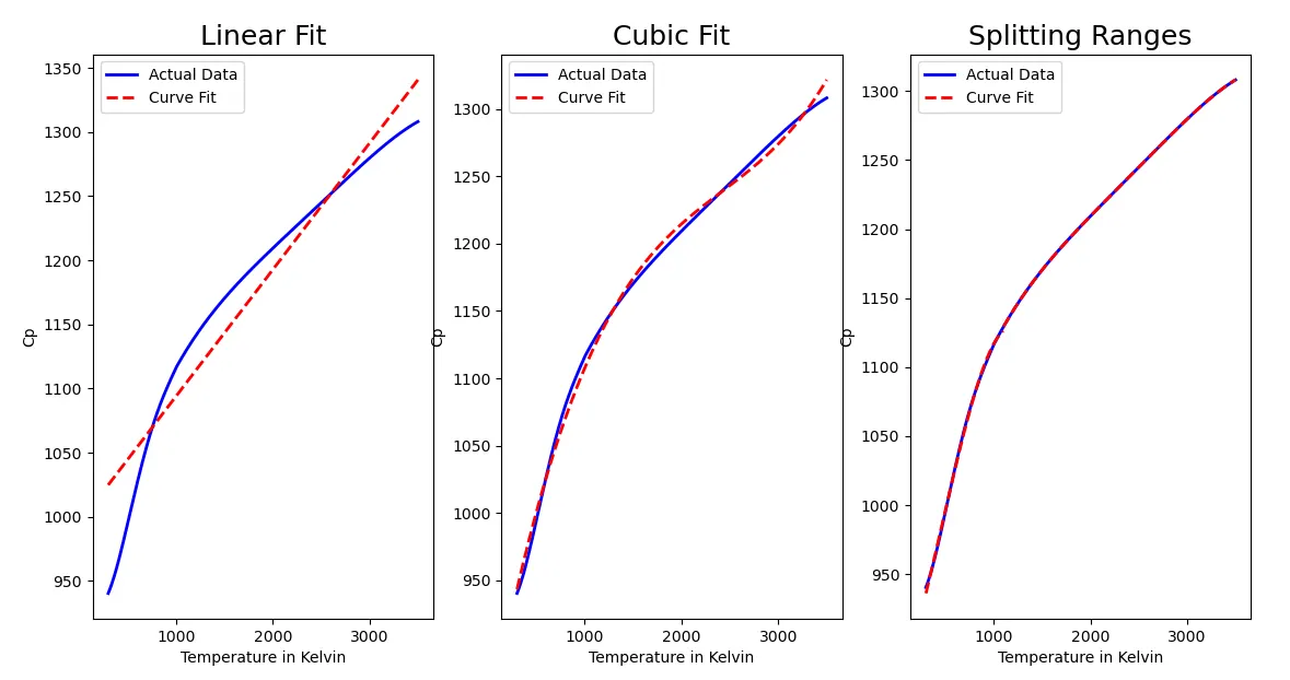
Therefore, from the results it can be concluded that by increasing the polynomial degree gives the good fit or splitting the range of the data given and performing curve fitting for individual dataset yields the best possible curve fit.