Week 4 - CHT Analysis on Exhaust port

AIM:-

• Brief Study on CHT analysis with why and where its uses.
• Calculate the Y+ value according to the turbulence model and simulate the final results.
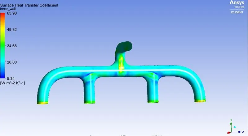
• Calculate the wall/surface heat transfer coefficient on the internal solid surface.
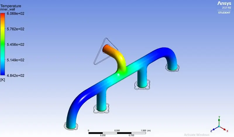
• Plot velocity and Temperature contours on the required area.
• Confirm, if the HTC prediction from the simulation is correct. Furthermore, state, on what factors does the accuracy of the prediction depends.

OBJECTIVE:-

• Understand the concept of the Conjugated heat transfer along with its applications.
• Prepare the geometry by generating fluid volume. In this case, we will require both fluid and solid volume to calculate the heat transfer coefficient between fluid and solid.
• Simulate the baseline simulation to get an idea about simulation setup and results.
• For the final result execute a fine mesh with proper inflation layer considering proper Y+ value.
• Simulate with both k-epsilon and k-omega turbulent models to check suitable simulation types.
• Plot both wall and surface heat transfer coefficient on the internal solid surface.
• Plot velocity and pressure contour on the required area of the exhaust port.
• Validate the results with mesh independence and get confidence over results by conducting some exact calculations at the inlet and outlet port.

CONJUGATE CONVECTIVE HEAT TRANSFER MODEL:

The contemporary conjugate convective heat transfer model was developed after computers came into wide use to substitute the empirical relation of proportionality of heat flux to temperature difference with heat transfer coefficient which was the only tool in theoretical heat convection since the times of Newton. This model, based on a strictly mathematically stated problem, describes the heat transfer between a body and a fluid flowing over or inside it as a result of the interaction of two objects. The physical processes and solutions of the governing equations are considered separately for each object in two subdomains. Matching conditions for these solutions at the interface provide the distributions of temperature and heat flux along the body–flow interface, eliminating the need for a heat transfer coefficient. Moreover, it may be calculated using these data.

The Conjugate Heat Transfer (CHT) analysis type allows for the simulation of heat transfer between solid and fluid domains by exchanging thermal energy at the interfaces between them. Typical applications of this analysis type exist as, but are not limited to, the simulation of heat exchangers, cooling of electronic equipment, and general-purpose cooling and heating systems.

APPLICATION:

Conjugate heat transfer problems, where the heat conduction in a solid region is usually coupled with the convection heat transfer in an adjacent fluid region, are of great significance in many practical applications, for example, the electronic circuit cooling, the design of thermal protection system for space vehicles, thermal insulation of nuclear reactor, turbine blade cooling, and solar panel design.

Conjugate Heat Transfer (CHT) is applicable whenever there are two adjacent domains and we wish to analyze the heat transfer between these domains. These domains can either be solid or fluid. One example is the forced or natural convective cooling of a heat-sink attached to active electronics components which generate heat

For many simulations of real-world engineering applications, the predictions of heat transfer properties are as important, if not more important, than the actual flow field. Such scenarios include simulations of heat exchangers, HVAC (Heating, Ventilation and Air Conditioning), combustion/burners, electronics cooling, and many more. In these applications, we are often interested in how heat moves through both the fluid and solid domains, and importantly the transfer of heat across the interface between adjacent domains.

PROCEDURE:-

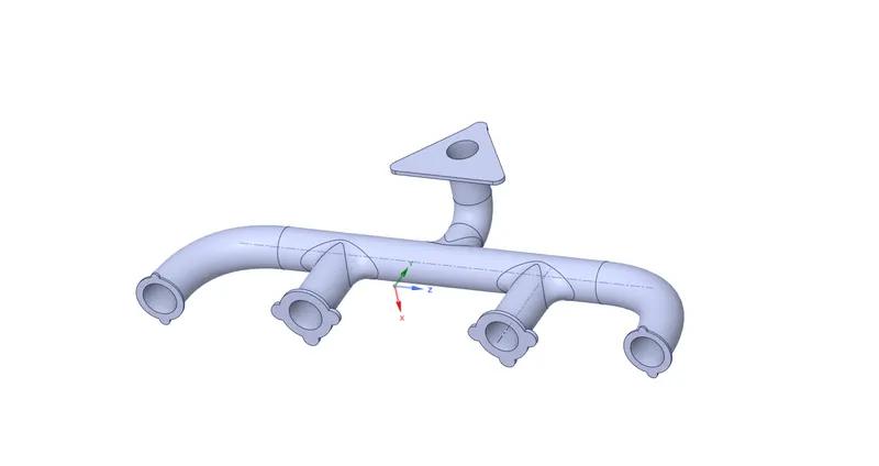
*The model is been downloaded and added to the fluent workbench and the geometry is been checked in the space claim

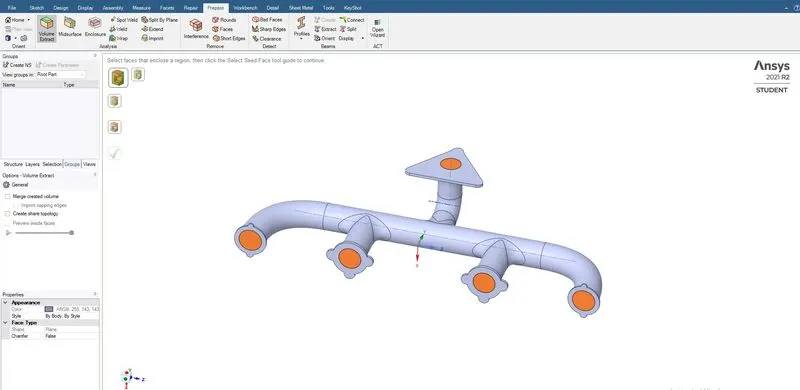
*The required area is volume extracted by selecting the edges of the inlets and outlet.

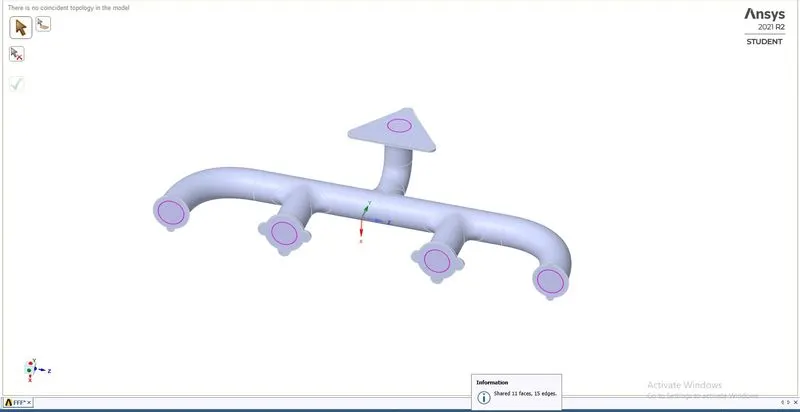
The volume are been checked share so mesh inflation can be done to interconnect the volumes.

BASE SETUP CASE

*The mesh is created for an element size of 150mm and the quality of the elements we more than 40%.

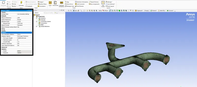
*The Setup workbench is started and given recommended parameters.

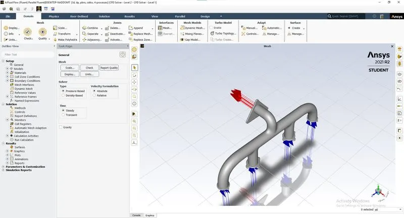
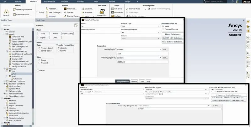
*The material is been added, the air is been initiated with specific values at both the inlets

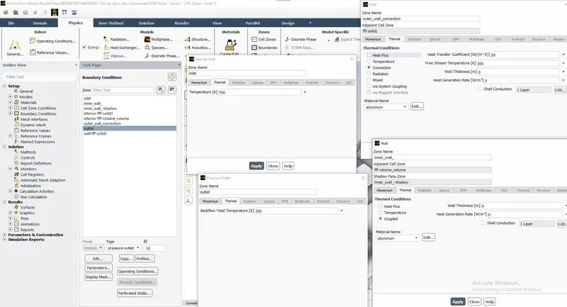
*Boundary Conditions are applied on the inlet with velocity values, outlet with pressure at zero, and the wall with No-slip conditions and with convection.

*Boundary Conditions are applied on the inlet with temperature values, outlet with the temperature at ambient condition.

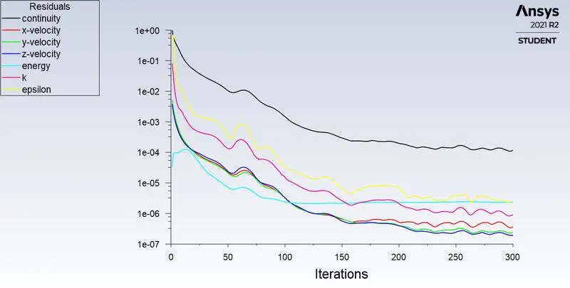
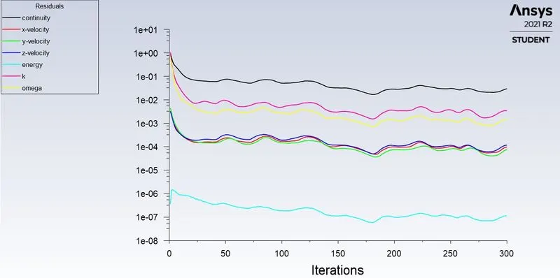
*The residuals, surface report of Area weighted average for heat transfer coefficient, and standard deviation at the inner wall, Pressure and Velocity contour are plotted to show the model has reached convergence.

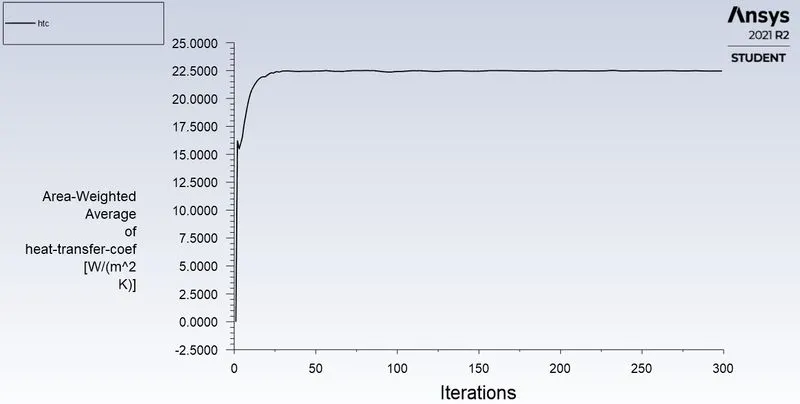
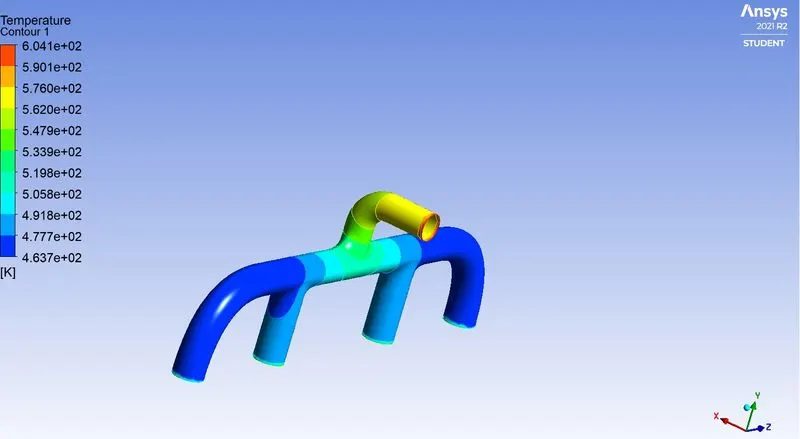
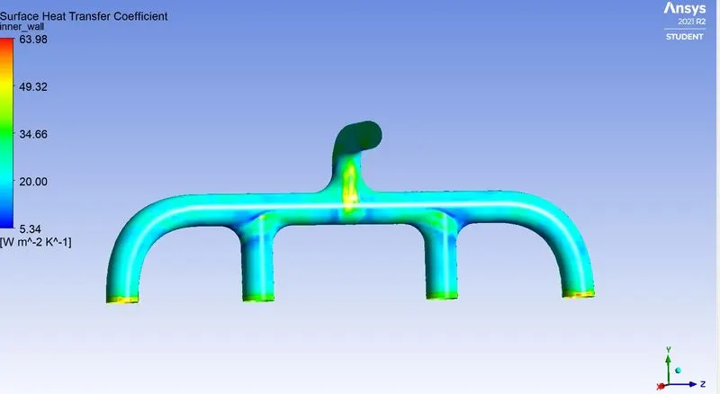
CASE

*The mesh is created for an element size of 0.15m and the quality of the elements we more than 40%, with Inflation layers Y+(3) for the mesh by 6 layers near the inner wall and outer wall region.

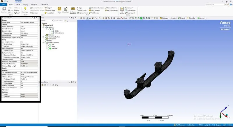
*The residuals, surface report of Area weighted average for heat transfer coefficient, and standard deviation at the inner wall, Pressure and Velocity contour are plotted to show the model has reached convergence.

RESULT:-

GRID INDEPENDENCE	NUMBER OF ELEMENTS	SURFACE HEAT TRANSFER COEFFICIENT `(W)/(m^2.K)`
Without Inflation layers	136101	22.535
With Inflation layers Y+(3)	281415	22.47

CALCULATION:-

Nussalt Number:-

`Nu=0.023*Re^0.8*Pr^0.4`

`Nu=(h*l)/(k)`

Reynolds number `=(rho*V*l)/(mu)`

`rho=1.225 (kg)/(m^3)`

V=`5m/s`

l=0.1661m

`mu=1.78e^-5(kg)/(m*sec)`

`Re=(1.225*5*0.1661)/(1.78e^-5)`

Re=57155.19.

For Air at `700 K`,

Pr=0.710.

k=`0.048(W)/(m*K)`

`Nu=0.023*(57155.19)^0.8*0.710^0.4`

`Nu=128.1963`

`h=(Nu*k)/(l)`

`h=(128.1963*0.048)/(0.1661)`

Surface Heat Transfer Coefficient `h=37.046(W)/(m^2*K)`

CONCLUSION: -

• The mesh is a very important parameter to get good results, that's why we have to refine it in the important place of our geometry .Mesh/ grid dependency test is very important.
• One factor that should be considered which is the most significant is the turbulent boundary layer. If we are using any kind of low Reynold’s turbulence model considering enhanced wall treatment (as our K-w SST model), so we need to make sure that we stay in the laminar sub-layer region where velocity profiles are assumed to be laminar and viscous stress dominates the wall shear which means (Y+<5)
• In the fluent software, the value of the convective heat transfer coefficient extremely depends on the reference temperature.