Aim :- To study the genetic algorithm & finding the global maxima of the function.

Theory:- In computer science and operations research, a genetic algorithm (GA) is a metaheuristic inspired by the process of natural selection that belongs to the larger class of evolutionary algorithms (EA). Genetic algorithms are commonly used to generate high-quality solutions to optimization and search problems by relying on biologically inspired operators such as mutation, crossover and selection.

Five phases are considered in a genetic algorithm.

1. Initial population
2. Fitness function
3. Selection
4. Crossover
5. Mutation

Initial Population

The process begins with a set of individuals which is called a Population. Each individual is a solution to the problem you want to solve.

An individual is characterized by a set of parameters (variables) known as Genes. Genes are joined into a string to form a Chromosome (solution).

In a genetic algorithm, the set of genes of an individual is represented using a string, in terms of an alphabet. Usually, binary values are used (string of 1s and 0s). We say that we encode the genes in a chromosome.

Fitness Function

The fitness function determines how fit an individual is (the ability of an individual to compete with other individuals). It gives a fitness score to each individual. The probability that an individual will be selected for reproduction is based on its fitness score.

Selection

The idea of selection phase is to select the fittest individuals and let them pass their genes to the next generation.

Crossover

Crossover is the most significant phase in a genetic algorithm. For each pair of parents to be mated, a crossover point is chosen at random from within the genes.

Mutation

In certain new offspring formed, some of their genes can be subjected to a mutation with a low random probability. This implies that some of the bits in the bit string can be flipped.

Matcode to solve the problem:-

% To solve the genetic algorithm equation for three studies

clear all
close all
clc

% Independent variable
x= linspace(0,0.5,150);
y= linspace(0,0.6,150);

%matrix
[xx,yy] = meshgrid(x,y);
% Number of iterations
num_cases = 50;
% starting the loop

for i = 1:length(xx);

    for j=1:lenght(yy)
        input_vector(1) = xx(i,j);
        input_vector(2) = yy(i,j);
        f(i,j) = stalagmite(input_vector);
    end

    % Create a three dimensional surface
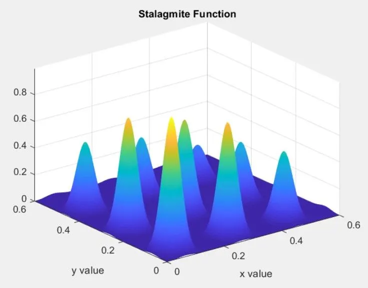
    figure(1)
    surfc(xx,yy,-f)
    shading interp %makes the surface look more smoother
    xlabel('x value')
    ylabel('y label')
    title('Stalagmite Function')

    % case 1 study
    tic
    for i=1:num_cases
        [inputs,fopt(i)] = ga(@stalagmite,2);
        xopt(i)= inputs(1);
        yopt(i)= inputs(2);

    end

% case_1 = toc
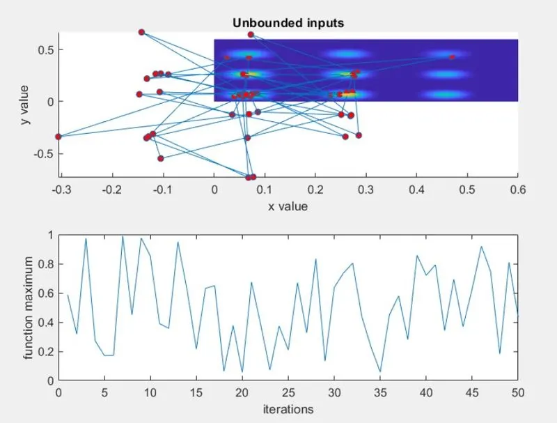
figure(2)
subplot(2,1,1)
hold on
surfc(x,y,-f)
title('Unbounder inputs')
xlabel('x value')
ylabel('y value')

shading interp
hold on

plot3(xopt,yopt,-fopt,'marker','o','Markersize',5,'Markerfacecolor','r')
subplot(2,1,2)
plot(-fopt)
xlabel('iterations')
ylabel('function maximun')

% case 2nd with upper and lower bounds

tic;
for i=1:num_cases

    [inputs,fopt(i)] = ga(@stalagmite,2[],[],[],[],[0;0],[0.6;0.6]);

    xopt(i) = inputs(1);
    yopt(i) = inputs(2);
end

% case_2_time = toc
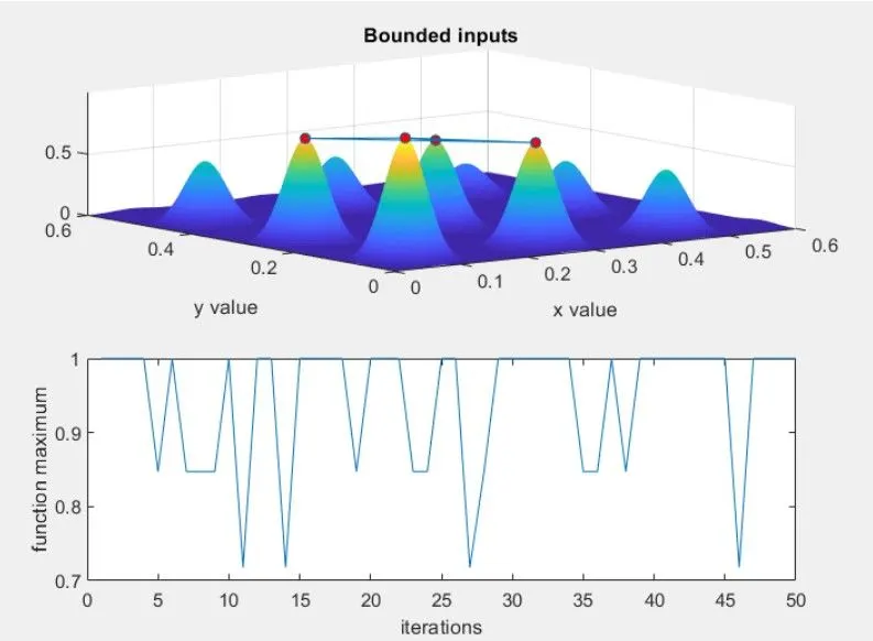
figure(3)
subplot(2,1,1)
surfc(x,y,-f)
shading interp

title('Bounded inputs')
xlabel('x value')
ylabel('y value')

hold on
plot3(xopt,yopt,-fopt,'marker','o','markersize',5,'markerfacecolor','r')
subplot(2,1,2)
xlabel('iterations')
ylabel('function maximun')

% case study 3 increasing the population size
% by doing so we are increasing the probability of the function
% to converge at global maximum

options = optimoptions(@ga)
options = options(@ga,'Populationsize',500)

% increasing the population size

tic
for i=1:num_cases
    [inputs,fopt(i)] = ga(@stalagmite,2,[],[],[],[],[0;0],[0.6;0.6],[],[],options);
    xopt(i) = inputs(1);
    yopt(i) = inputs(2);

end
% case_3_time = toc 
%gives the time taken for study
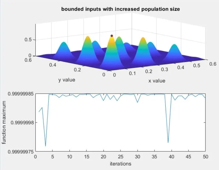
figure(4)
subplot(2,1,1)
surfc(x,y,-f)
%creates a surface to visualise 3D
shading interp
title('bounded inputs with increased population size')
xlabel('x value')
ylabel('y value')

hold on
plot3(xopt,yopt,-fopt,'markersize',4,'markerfacecolor','r')
subplot(2,1,2)
plot(-fopt)
%plotting -f vs number of iterations
xlabel('iterations')
ylabel('funation maximun')

Function code to solve the equation:-

% function code
function[f] = stalagmite (input_vector);

a = input_vector(1);
b = input_vector(2);

term1 = (sin((5.1*pia)+0.5))^6;
term2 = exp(-4*log(2)*((a-0.0667)^2)/0.64);
term3 = (sin((5.1*pi*b)+0.5))^6;
term2 = exp((-4)*log(2)*((b-0.0667)^2)/0.64);

[f] = (term1*term2*term3*term4);

%inverts the objective function
end

Grapical output of program:-