Week 3 - Solving second order ODEs

AIM: To write a Python program that solves the Ordinary Differential Equation (ODE).

OBJECTIVES: 1) To write a program to solve 2^nd order ODE which represents the equation of motion of a simple pendulum with damping.

                      2) To write a program that will simulate the pendulum motion between 0 to 20 sec to create an animated movie.

EQUATION

                      The primary equation use in this topic is as following;

`(d^2 theta)/(dt^2 )+ b/m d(theta)/dt+ g/l sintheta =0`

Where,

          g = gravity in m/  

          l = length of the pendulum in m,

          m = mass of the ball in kg

          b = damping coefficient

This is a 2^nd order ODE that is used in this topic to determine the pendulum motion.

THEORY :

                        A simple pendulum described ideally as a point mass suspended by a massless string from some point about which it is allowed to swing back and forth in a place. A simple pendulum can be approximated by a small metal sphere that has a small radius and a large mass when compared relatively to the length and mass of the light string from which it is suspended. If a pendulum is set in motion so that is swings back and forth, its motion will be periodic.

                                                               

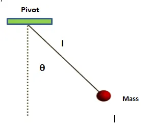
                                                                       Fig: Simple Pendulum

Simple pendulum motion helps us in the following manner;

1) To study the simple harmonic motion

2)To learn the relationships between the period, frequency, amplitude, and length of a simple pendulum.

INPUT PARAMETERS :

                    Damping coefficient , b = 0.05

                    Acceleration of gravity, g = 9.81 m/

                    Length of the pendulum , l =  1 m

                    Mass attached , m = 1 kg

                    Velocity = 3 rad/s

PROGRAM CODE:

1) Main Program

Programming Language: Python

# Program for solving second order ODEs and simulate its motion
import matplotlib.pyplot as plt
import math
from scipy.integrate import odeint
import numpy as np

# calling function
def model(theta,t,b,g,l,m):
 theta1=theta[0]
 theta2=theta[1]
 dtheta1_dt=theta2
 dtheta2_dt=-(b/m)*theta2-(g/l)*math.sin(theta1)
 dtheta_dt=[dtheta1_dt,dtheta2_dt]
 return dtheta_dt

# Inputs
# damping coefficient
b = 0.05
# acceleration due to gravity(m/s^2)
g = 9.81
# length of string (m)
l = 1
# mass of bob (kg)
m = 1
# Initial Conditions
theta_0 = [0,3]
# time points
t_span = np.linspace(0,20,100)
# Solve ODE
theta = odeint(model,theta_0,t_span,args = (b,g,l,m))
# Plotting the graph
plt.plot(t_span,theta[:,0],'b-',label=r'$\frac{d\theta1}{dt} = \theta2$')
plt.plot(t_span,theta[:,1],'r--',label=r'$\frac{d\theta2}{dt} = -\frac{b}{m}\theta2 - \frac{g}{l}sin\theta1$')
plt.xlabel('Time (second)')
plt.ylabel('Plot')
plt.title('Damped Harmonic motion of a Simple Pendulum')
plt.legend(loc='best')
plt.ylim([-3.5,3.5])
plt.xlim([0,20])
plt.grid()
plt.show()
# Iteration using for loop to create animation of motion of pendulum
ct =1
range = theta[:,0]
for i in range:
  x_start = 0
  y_start = 0
  x_end = l*math.sin(i)
  y_end = -l*math.cos(i)
  # Plotting for animation
  plt.figure()
  # Plotting the rigid support through which string of pendulum is attached
  plt.plot([-0.5,0.5],[0,0],linewidth=3)
  # Plotting String of pendulum
  plt.plot([x_start,x_end],[y_start,y_end],linewidth=4)
  # Plotting Bob of pendulum
  plt.plot(x_end,y_end,'o',markersize=25)
  plt.xlim([-1.0,1.0])
  plt.ylim([-1.2,0.2])
  
  filename = 'test%05d.png' % ct + '.png'
  plt.savefig(filename)
  ct = ct + 1

OUTPUT:

1)Graph of the effect of Damping

 

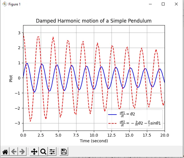
2)Pendulum motion animation:

https://drive.google.com/file/d/1hISk0xmtNN5BZXGTLFOI1AzzCKyAjROQ/view?usp=sharing 

CONCLUSION:

                      The output for angular displacement & angular velocity is obtained for a simple pendulum. Also, animated simulation is created with the help of a Python program.