Week 3: Flow over a backward facing step
Aim:
Simulate flow through a backward facing step (BFS) and post process the results for 3 base mesh sizes 1e-3m,1.5e-3m & 2e-3m.
Theory:
Backward Facing Step
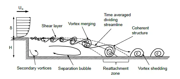
Flow through a BFS is an example of seperation flow as the flow gets seperated at the step of the BFS.The sepreated flow occurs mainly due to the sudden change in the geometry. Flow Seperation occurs because the boundary layer can no longer follow the profile of the channel hence the boundary layer seperates at a seperation point forming vortices.The wake of the flow is characterized into 3 regions 1.seperation bubble 2.shear layer region 3.reattatchment zone.
1.Seperation Bubble
The separation bubble contains large vortex that posses a low circulation velocity.It is trapped between the shear layer and reattatchment zones.
2.Shear layer region
The shear layer contains a mixture of turbulent structures (vortices) within and increases in size with downstream flow.It occurs due to the velocity gradient between free stream flowing above and low velocity of circulation region.
3.Reattatchment zone
The reattatchment zone is the area where the shear layer merges with the wall.The distance between the step and reattatchment point is called reattatchment length.
Parameters that affect the above 3 are :1.aspect ratio (width of step/height) 2.Expansion ratio (total height/step height) 3.Free stream velocity 4.Reynold's number
Navier Stokes Equation
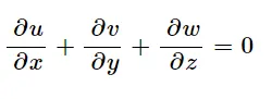
The solution for the simulation is obtained by solving the navier stokes equation. It is a set of equation consiting of 1 continuity equation , 3 momentum equation for 3 directions of velocity and 1 energy equation. The energy equation is applicable only in the case of heat transfer flows.
Equations for incompressible flow
Continuity Equation
Momentum Equations
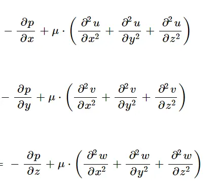
Here we have 4 equations and 4 unknowns (pressure,3 velocity components) which can be solved with a system of linear equations. In this project we use the PISO algorithm to solve the linear equations.
1.Pre-Processing
1.1 Geometry
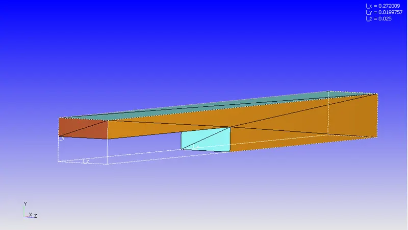
The backward facing step geometry has the dimensions x=0.27m y=0.019m & z=0.025m
1.2 Boundary flagging
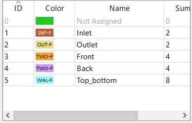
The various boundaries for the BFS is assigned.
2.Case Setup
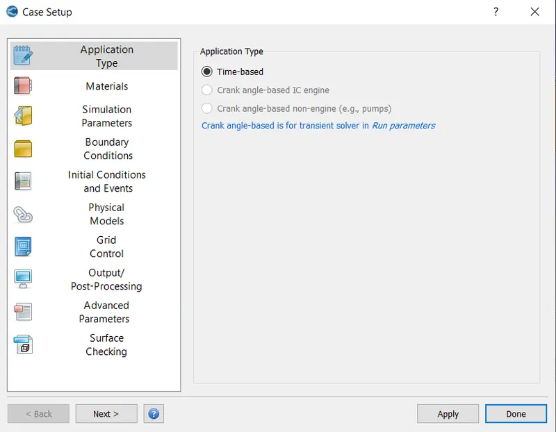
2.1 Application Type
The application type is taken as time based.
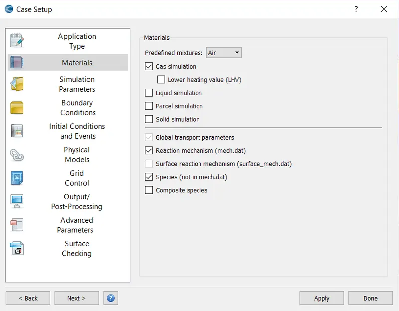
2.2 Materials
Under materials the predefined mixture air is selected as working medium.The values for gas simulation,global transport phenomena,reaction mechanism and species is taken as default.
2.3 Simulation parameters
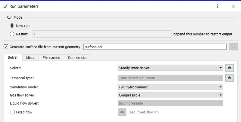
2.3.1 Run parameter
Under run parameter the simulation type is taken as full hydrodynamic as we need to solve the navier stokes equation to obtain the results as opposed to non hydrodynamic which only generates the mesh.Full hydrodynamic can be used for simpler structures like the BFS.
The solver is choosen to be steady state.
2.3.1.1 Steady state monitor
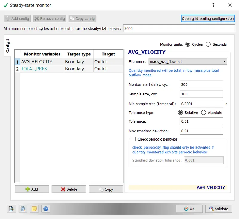
Under run parameters the steady state monitor is checked this allows us to monitor the convergence of necessary variables and hence can complete the simulation when the variables have converged allowing for faster simulation.
Here the average velocity and total pressure at outlet is monitored.
Minimum number of cycles is given as 5000 . This means that the simulation will run for atleast 5000 cycles before terminating when convergence is reached.
2.3.2 Simulation time parameters
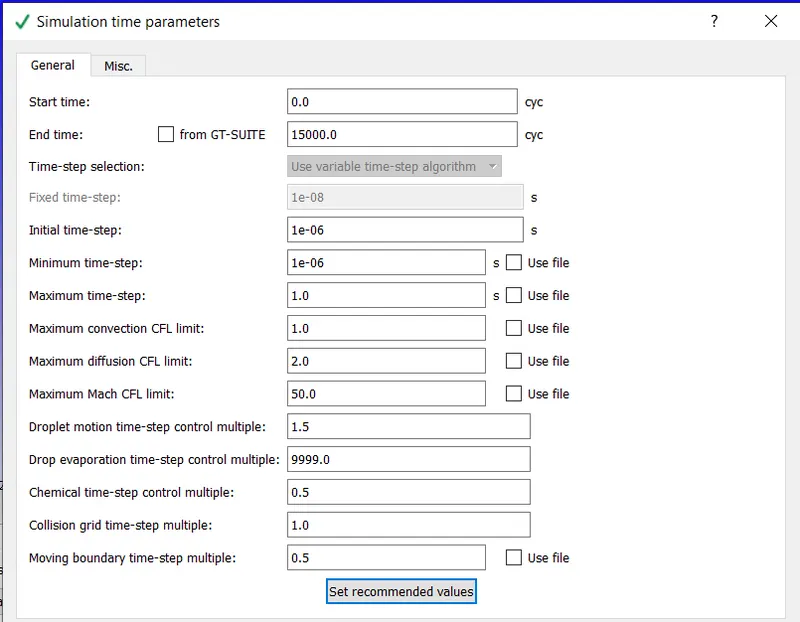
The start time is taken as 0.0 cyc and end time is 15000 cyc
Initial and max time step are 1e-6s and 1s respectively
2.3.3 Solver parameters
The solver scheme is PISO and the solver type is taken as pressure based.
2.4 Boundary conditions
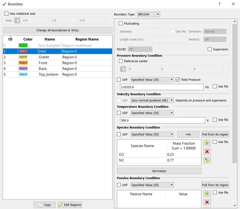
Each boundary flagged in the geometry is given the boundary conditions and all boundaries are assigned a region.
Inlet:The type is inflow , Total pressure = 110325 Pa and the medium is air
Outlet:The type is outflow , Static pressure = 101325 Pa and medium is air
Top_bottom:The condition is wall
Front and back:The condition is 2D
2.5 Regions and Initialization
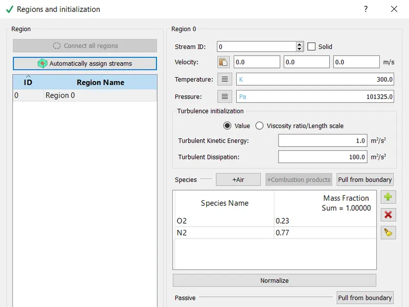
The inital pressure is 101325.0 Pa and the region is filled with air.
2.6 Physical Model
The model used is RANS_K_EPS_RNG
2.7 Grid control
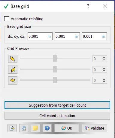
2.7.1 Base grid
The grid is set to 3 test cases for 3 simulation 1e-3m,1.5e-3m,2e-3m.
2.7.2 Fixed Embedding
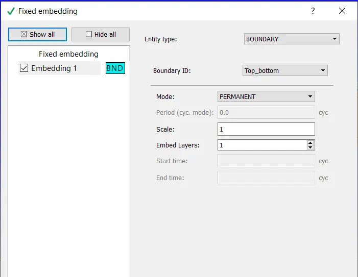
Fixed embedding is given for a finer mesh at the walls to increae the accuracy of the solution at the walls.
Post Processing
The post processing is done after the conversion of the .out files obtained vtk in line binary files and then viewing them in paraview software.
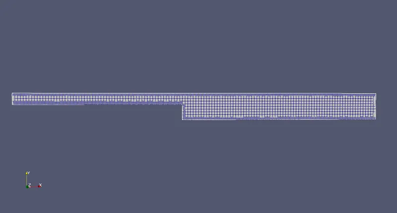
1. For 2 e-3m mesh size.
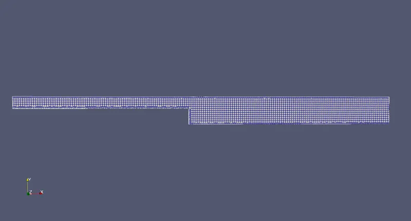
Grid
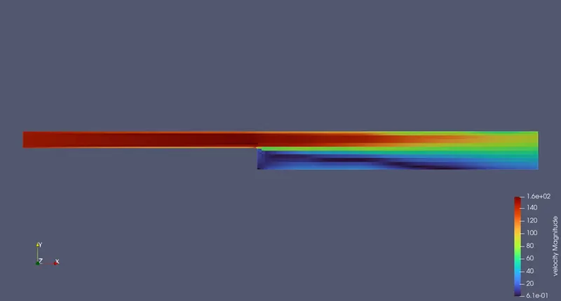
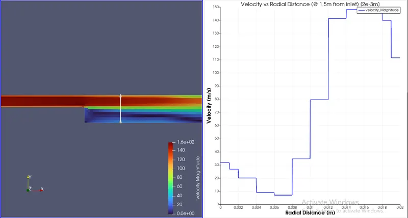
Velocity contour
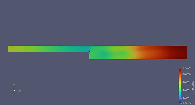
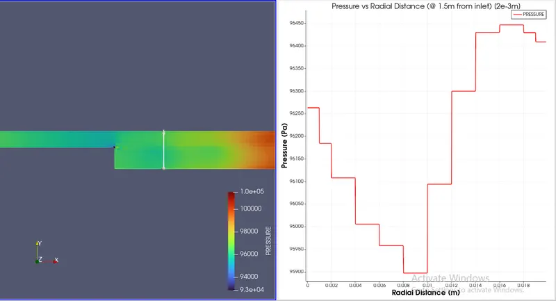
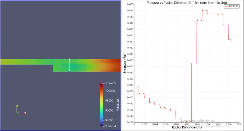
Pressure distribution
2. 1.5e-3 m
Grid
Velocity contour
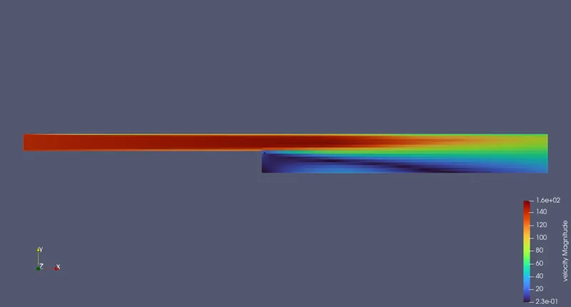
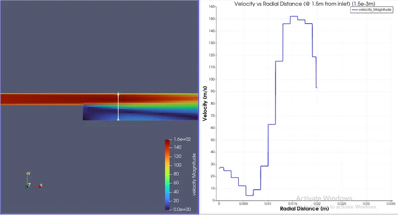
Pressure Distribution
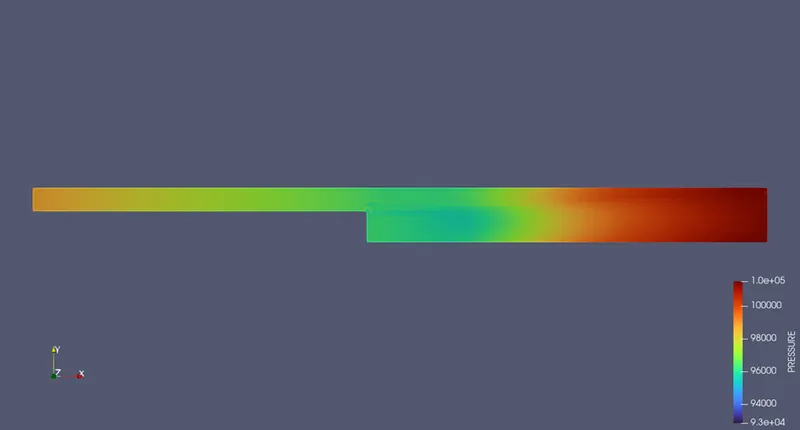
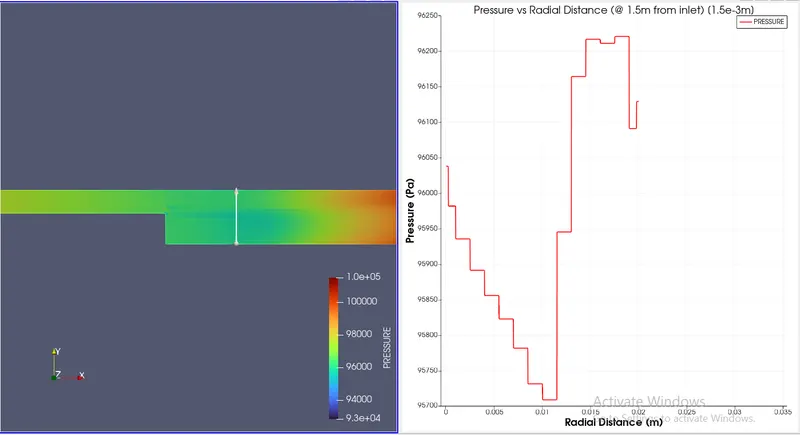
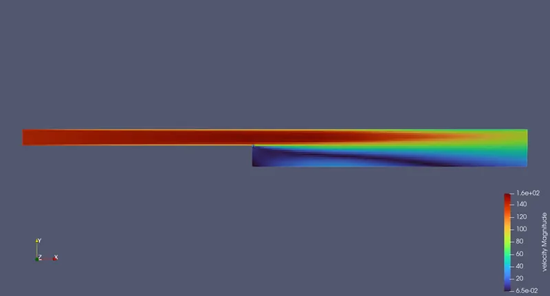
3. 1e-3 m
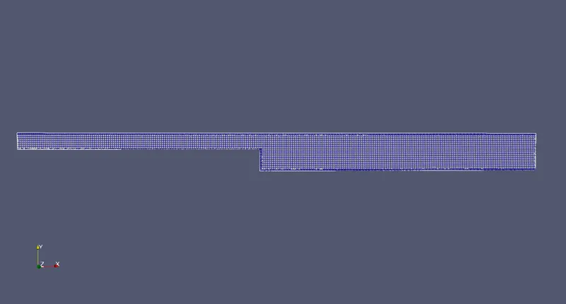
Grid
Velocity contour
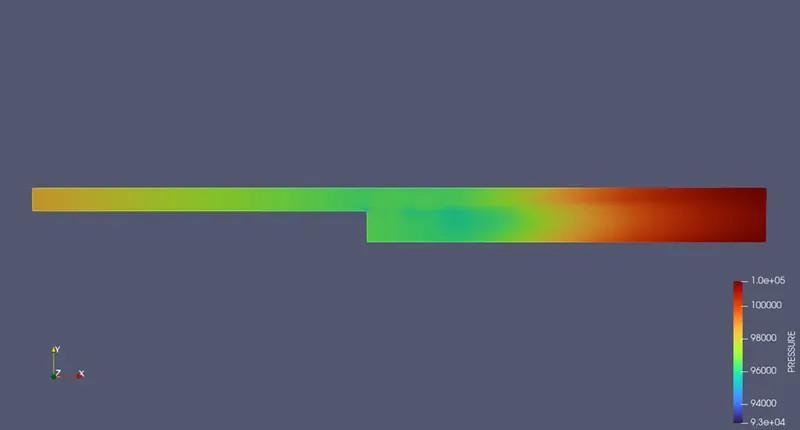
Pressure Distribution
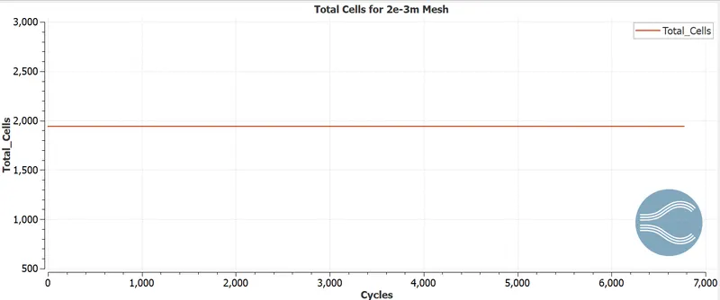
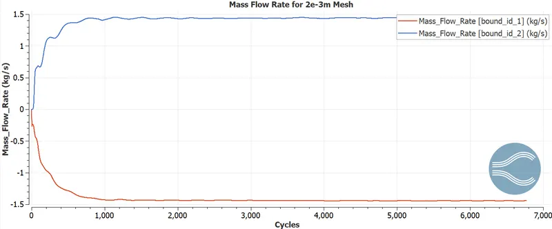
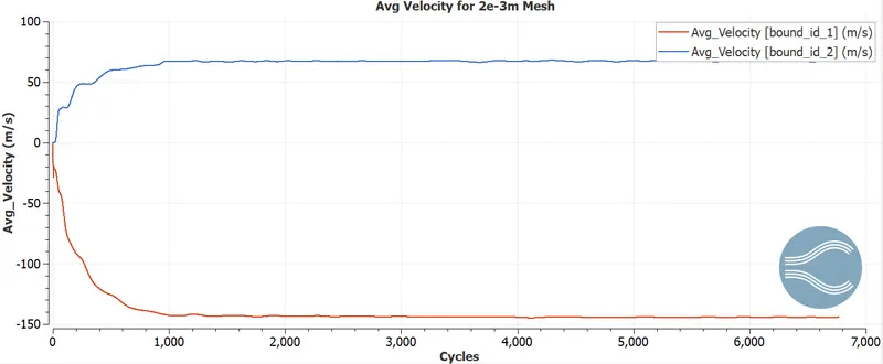
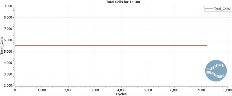
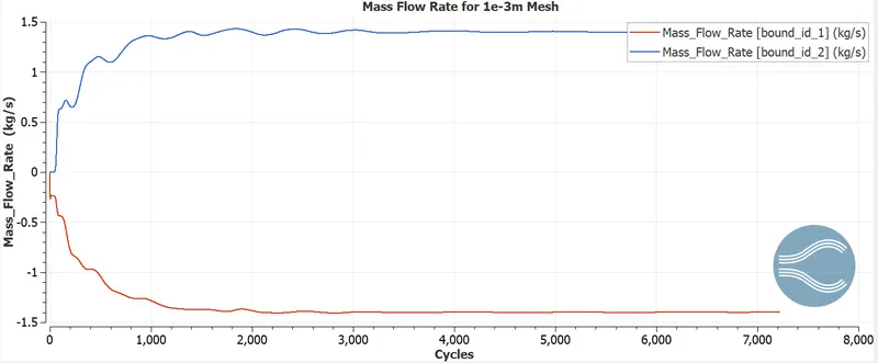
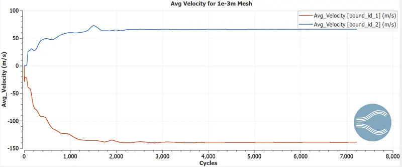
Converge Plots
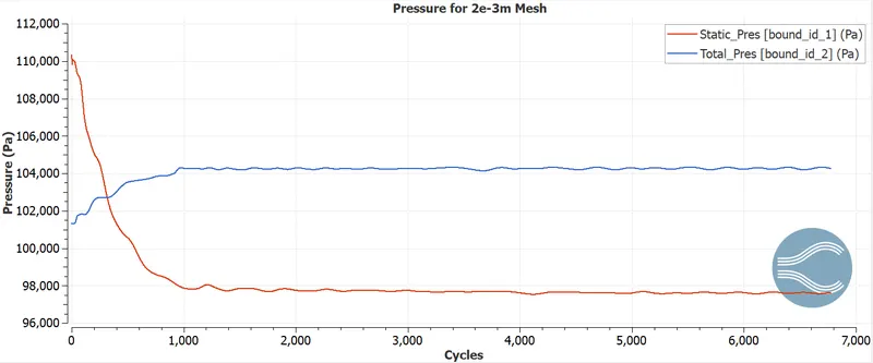
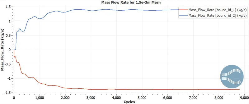
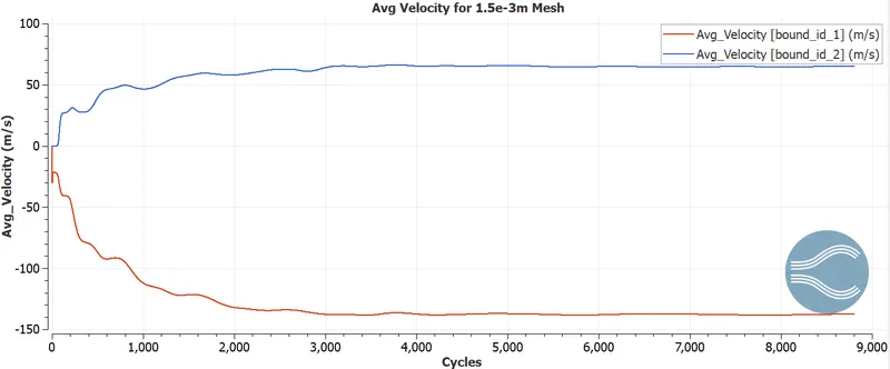
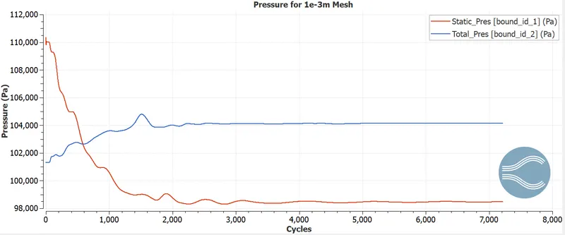
Here bound_id_1=inlet and bound_id_2=outlet
1. 2e-3m
2. 1.5e-3m
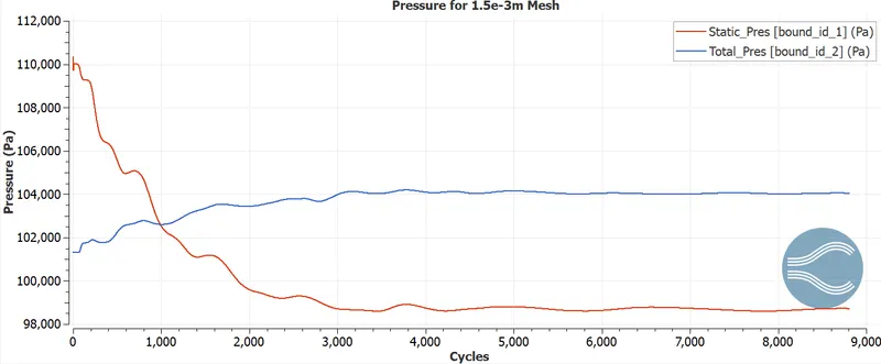
3. 1e-3m
Final flow vectors for 1e-3m
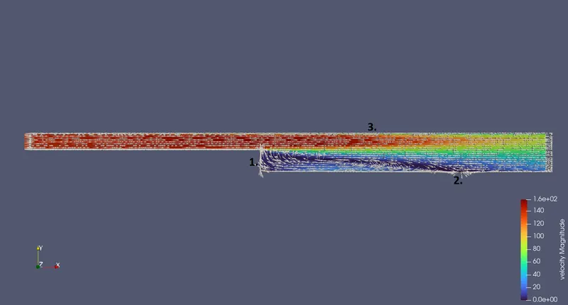
We can see the
1.Recirculation Bubble
2.Reattatchment zone
3.Free flow downstream
Flow Simulation
Flow Seperation
As the boundary layer reaches the step , there are 2 conditions that occur
`(delu)/(dely)=0`
`(delp)/(delx)>0`
the wall shear stress becomes zero and there is an adverse pressure gradient which decrease the speed of the flow , as a result the flow seperates from the step not being able to follow the profile of the step.
Observations:
1. We can see that the simulation coresponds to the actual phenomena when a flow through BFS occurs with formation of the recirculation bubble, shear layer and reattatchment layer.
2. For average velocity,pressure,mass flow rate we can observe that all 3 variables for all 3 base mesh size have reached convergence roughly about 6700 ~ 9000 cycles.
3.We can observe the embedding in the grid profile where the mesh at the walls are finer than the rest.
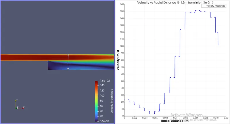
4. (i) From the above velocity graph we can observe that from a point 0.15 m away from inlet as we move radially upward the velocity starts to decrease, this is the recirculation bubble that contains low circulation velocity vortex (blue region).
(ii) As we go higher up we reach the shear region which has a higher velocity due to vortices. (green region)
(iii) As we further go higher radially we reach the free stream travelling downstream (red region) in which the velocity increases and then decreases (parabolic) typical of boundary layer flow through pipes.
5.Pressure distribution : Pressure begins to decrease as we move from left to right and then begins to increase till it reaches the maximum pressure (1041 Pa) .This increase in pressure is the adverse pressure gradient that pushes the flow of boundary layer backwards causing the recirculation bubble.