Week 1: Channel flow simulation using CONVERGE CFD
Aim:
In this project we will be setting channel flow using converge software with air as the medium.The simulation is run for 3 different mesh sizes. The mass flow, velocity,pressure and total cell count count w.r.t number of cycles is obtained from converge plot for all 3 mesh sizes.Velocity and pressure distribution is post processed using paraview software.
Theory:
Flow through pipes
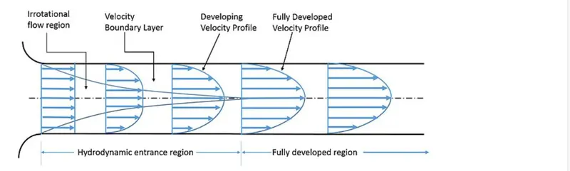
Boundary Layer
The region where the viscous shearing forces are felt and where velocity changes are significant along the radial direction is called boundary layer.The region where shearing forces due to the viscosity of the fluid is not felt and velocity is constant along the radial direction is called as irrotational flow region.
Hydrodynamic entrance length(Lh).
The distance from the inlet of the pipe to a point where the flow of the fluid is fully developed i.e after the hydrodynamic length the velocity profile of the fluid remains unchanged.
1.Geometry Creation
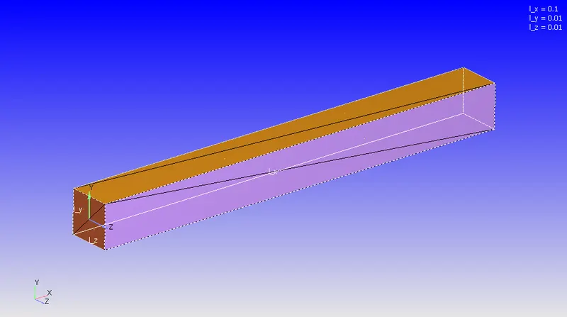
A channel having dimensions x=0.1m,y=0.01m & z=0.01m is constructed in converge.
Geometry->Create->Shape->Box
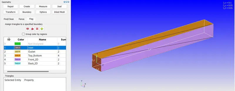
1.1. Boundary Setup
The differnet boundaries for the model is set.
2.Case Setup
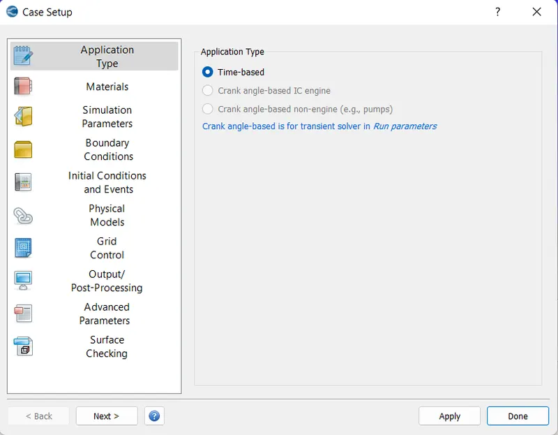
2.1 Application Type
The application type is choosen as time-based.
2.2. Materials
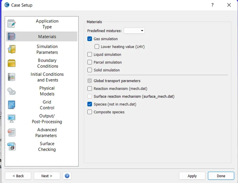
In materials gas simulation and species are selected (simulation of flow of air).
2.2.1 Gas Simulation & GLobal transport phenomena
The values are left as default.
2.2.2 Species
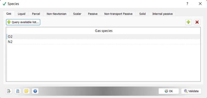
Under species O2 and N2 (Oxygen and Nitrogen) are selected as species present in the medium i.e air.
2.3 Simulation Parameters
2.3.1 Run parameters
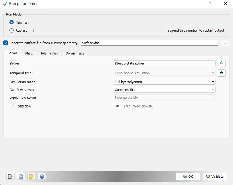
Under run paramters solver is choosen as steady state (since the simulation is a steady state analysis) and the simulation mode is fully hydrodynamic (since we want to solve the Navier Stokes equation as well apart from creating the mesh).
2.3.2 Steady State Monitor
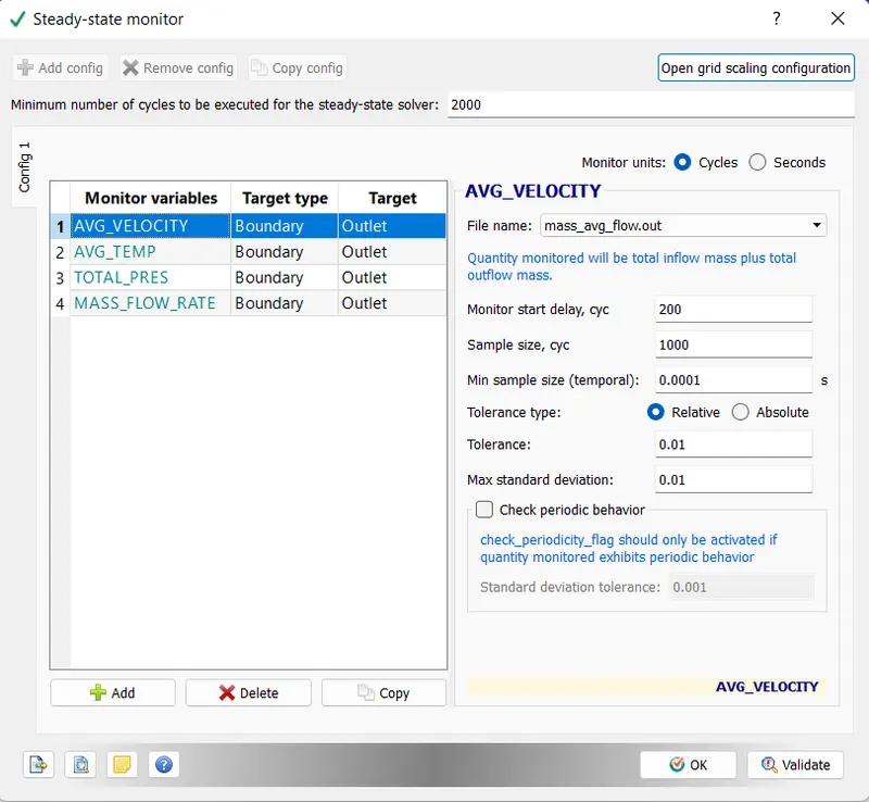
Under steady state monitor . The variables that need to be monitored for the simulation are selected.The simulation starts to check if these mentioned values have converged and if the values have converged then the simulation stops without having to go through the entire number of cycles (15000).
The value 2000 is provided to inform the solver that atleast 2000 cycles have to be performed for the simulation . The simulation will not terminate before 2000 cycles even if the values are converged.
The value 200 is the number of cycles the after which the variables start to be monitored.
The value 1000 is the sample size of values for which convergence is checked.
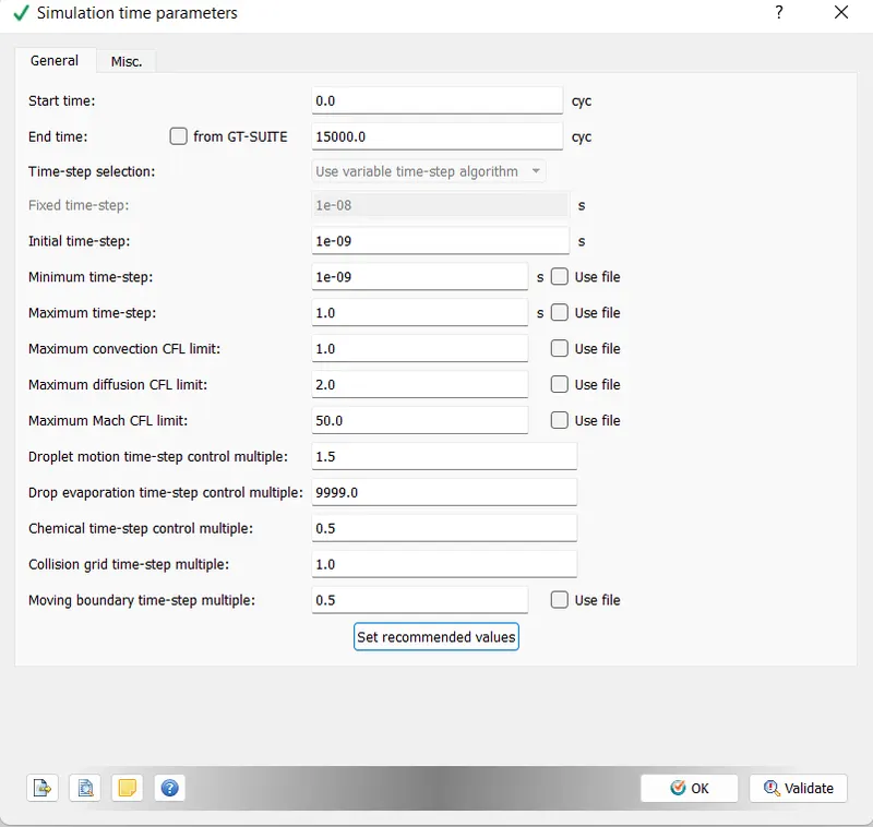
2.3.3 Simulation Time Parameter
Here the maximum number of cycles required for the simulation is provided (since this is a steady state simulation) =15000 & the value of time step in seconds = 1e-09 s.
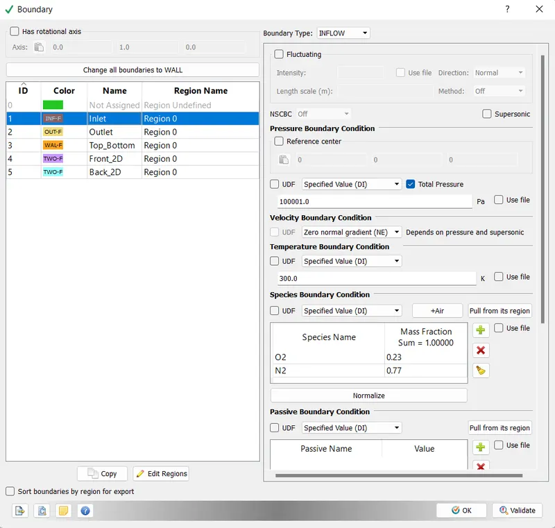
2.4 Boundary Conditions
The boundary conditions for the different boundaries are given.
Inlet: Pressure=100001 Pa , Species=O2 & N2
Outlet:Pressure=100000 Pa,Species=O2 &N2
Top & Bottom = No slip boundary condition (i.e. fluid velocity is zero)
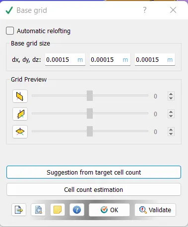
2.5 Base Grid
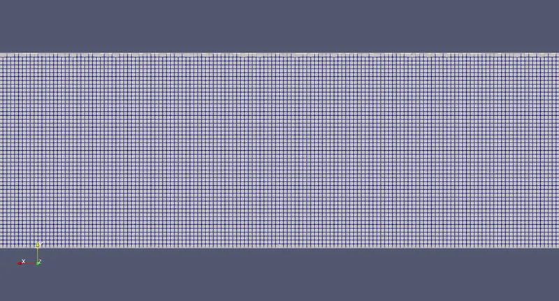
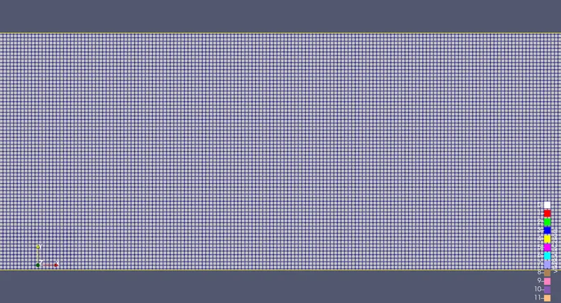
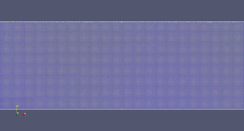
The mesh values are given dx,dy,dz (dz does not contribute since the simulation is only 2D)
2.5 Post Processing
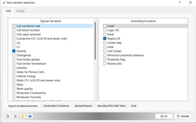
2.5.1 Post variable selection
The variables to be post process are selected.
2.5.2 Output Files
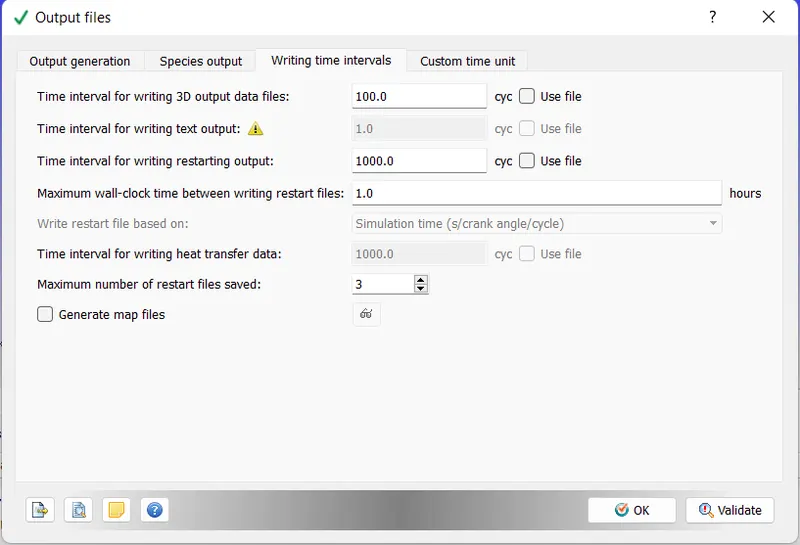
100 cycs is given so that for every 100 cyc a 3D output file is written (15000/100=150 3D files)
1000 cycs is given so that for every 1000 cyc a retsart file is written & the number of restart files is set to 3 which means only the last 3 restart files will be available.
3.Post Processing Results
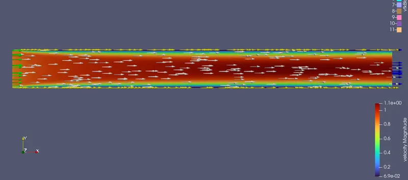
The post processing is done using paraview software. Tools like slice,plot over line is used to obtain the below post processing results.
Air flow thorugh the duct
1.For mesh size 2e-4m
Mesh
Velocity Profile
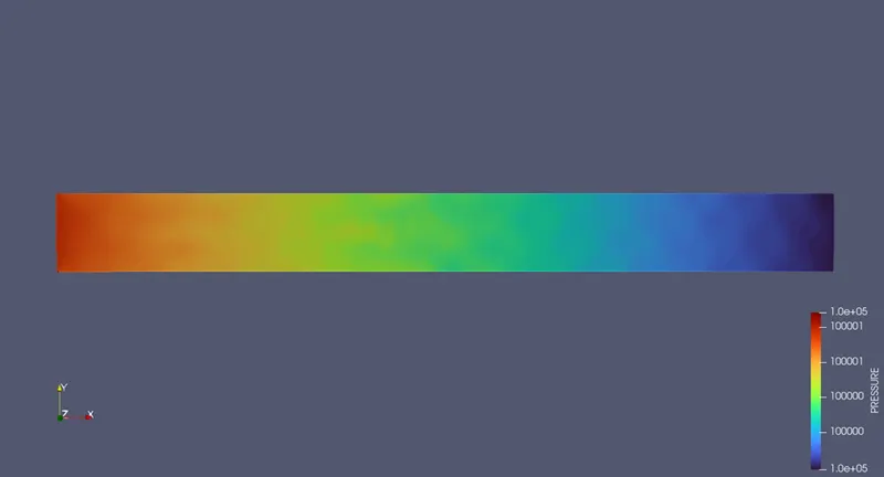
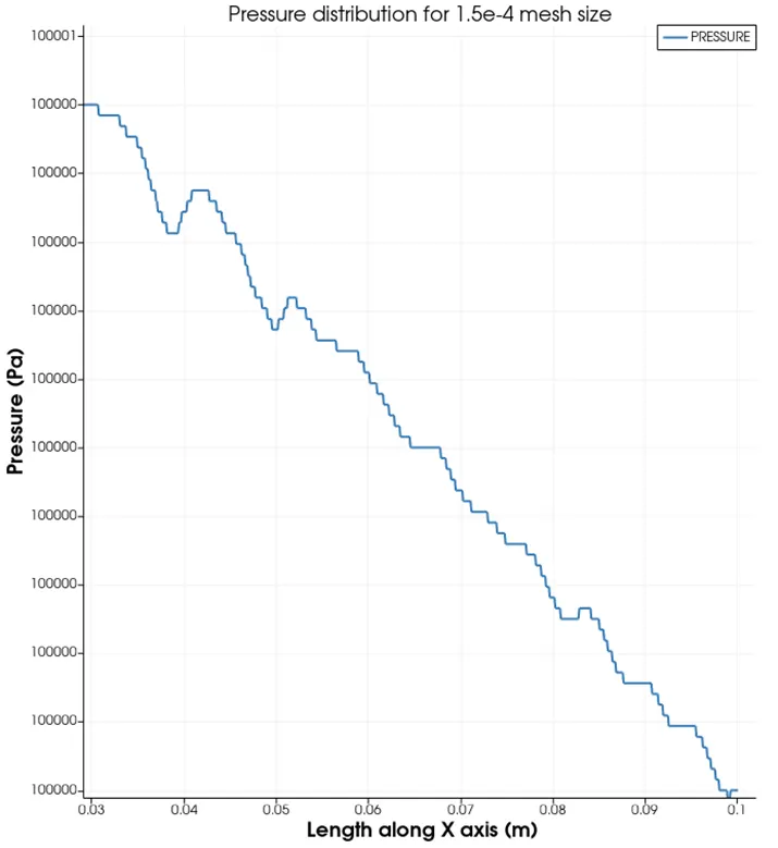
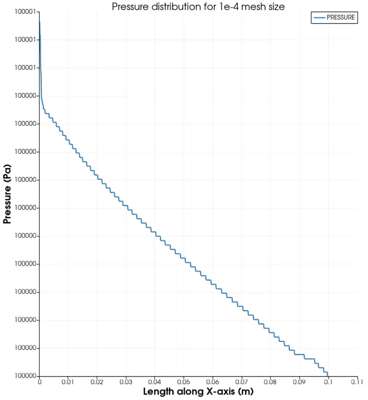
Pressure Distribution
2.For mesh size 1.5e-4
Grid
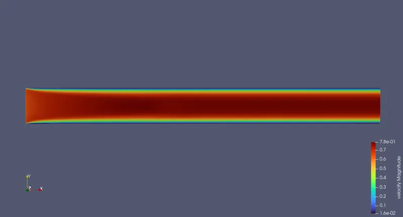
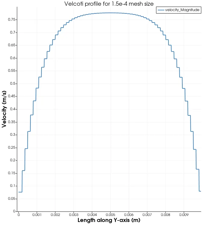
Velocity profile
Pressure Distribution
3.For mesh size 1e-4
Grid
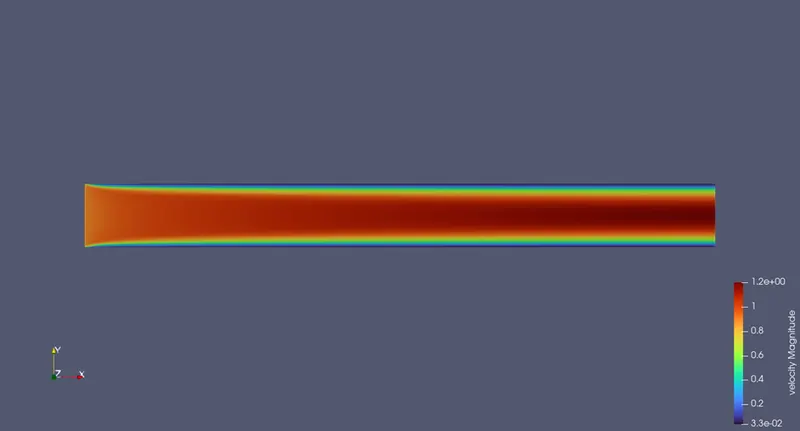
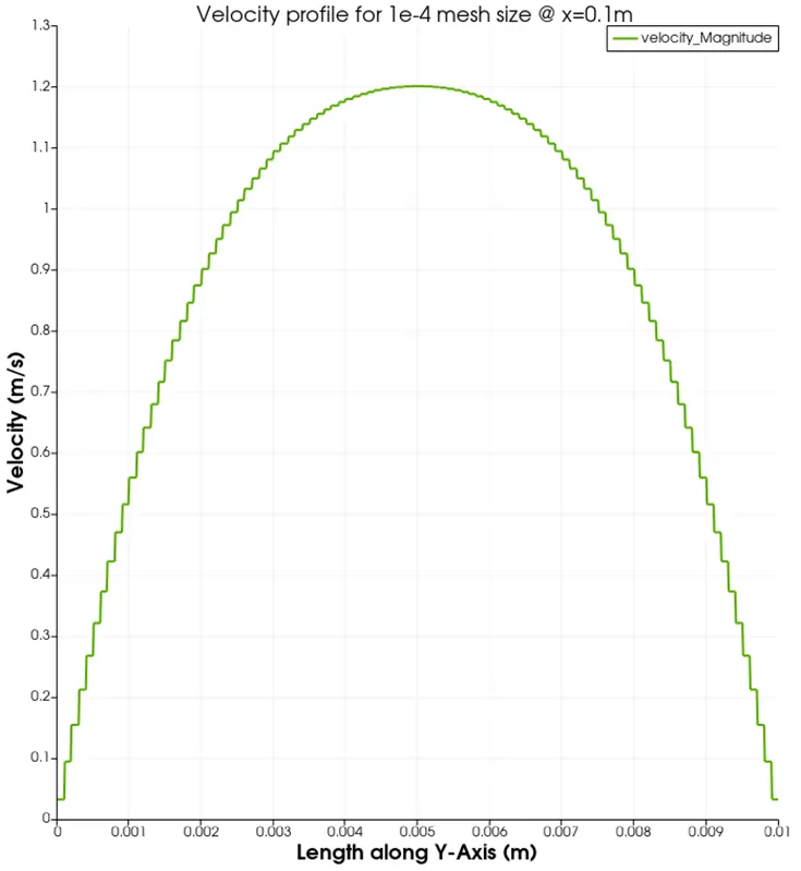
Velocity Profile
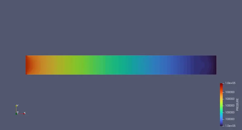
Pressure Distribution
Converge plots
1.Cell count
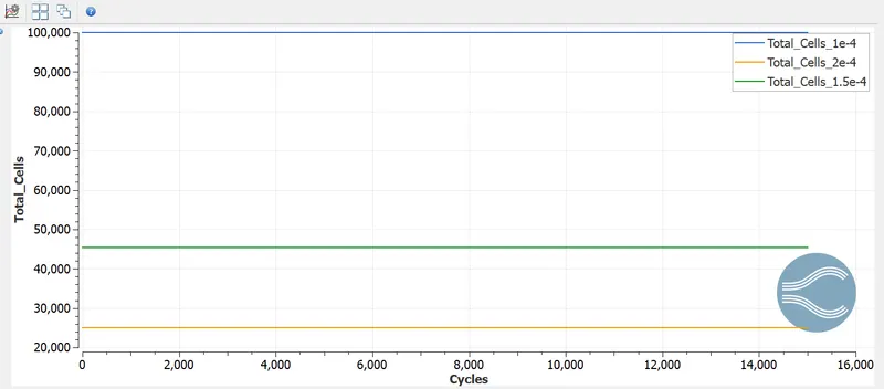
For mesh size of 1 e-4
No of cells in Y direction
`(0.01/0.0001)=100`
No of cells in X direction
`(0.1/0.0001)=1000`
Total cells
`100*1000=100000`
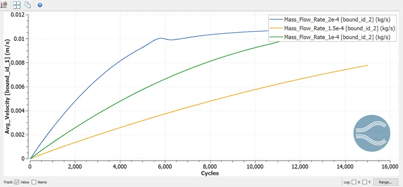
2.Mass flow rate [outflow]
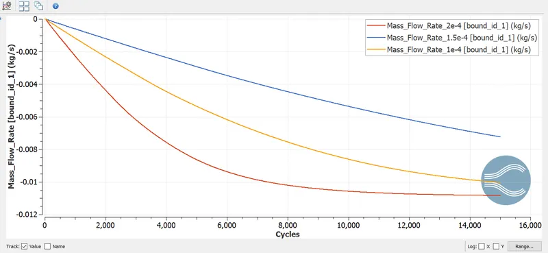
Mass flow rate [inflow]
3.Pressure
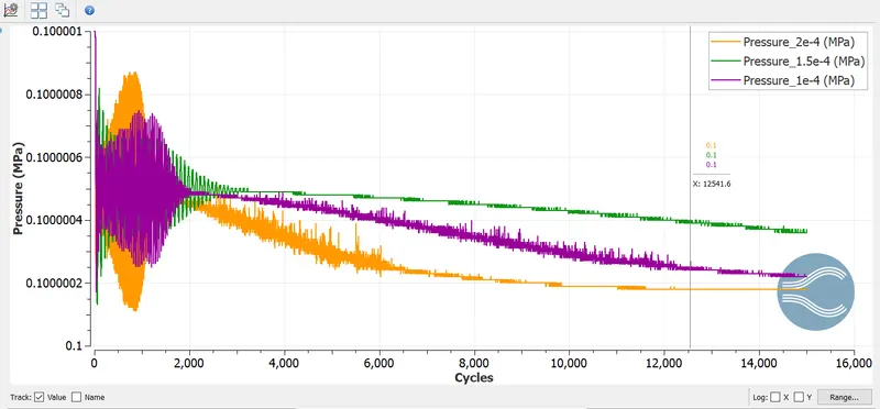
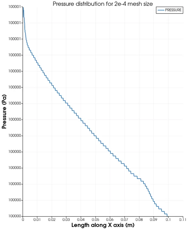
The plots for pressure for all 3 mesh sizes have converged to a value of 0.1 MPa
4.Velocity [inflow]
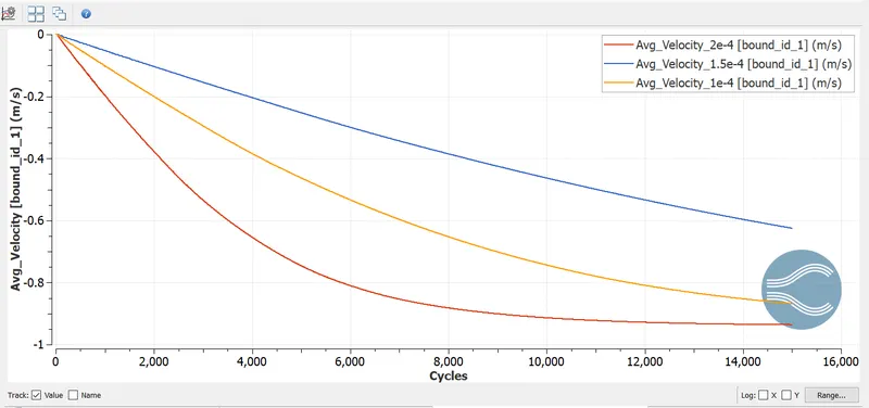
Simulation of channel flow [Velocity profile]
Observations
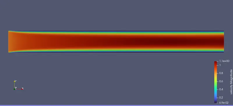
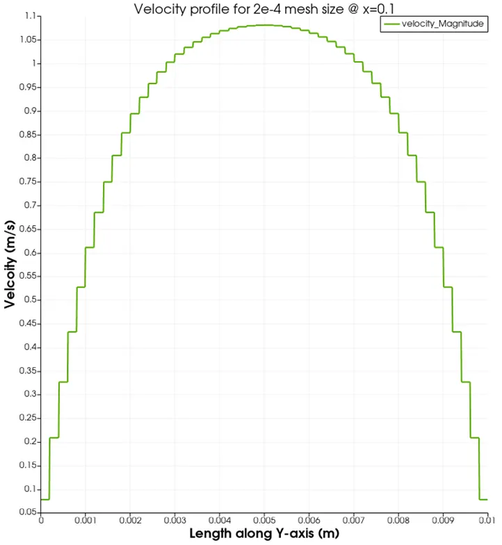
1) The flow inside the channel is laminar as the velocity profile for all 3 mesh sizes is a parabolic one as compared to a turbulent one which is more fuller.
2) Computational time was greatest for 1e-4 mesh size and least for 2e-4 mesh size as time increases with decrease in mesh size.
3) The graph for mass flow rate is symmetrical about X axis signifying the conservation of mass.
4) The steps in the velocity and pressure plots seem to smoothen out with decreasing mesh size.
Flow Description
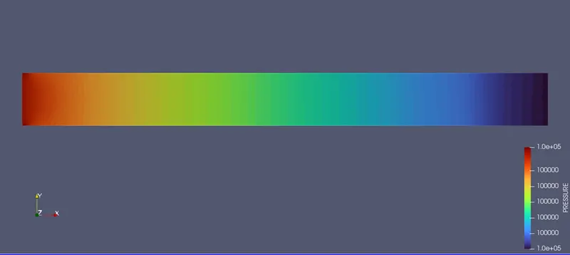
1)The flow starts with the inlet pressure as 100001 Pa and the outlet as 100000 Pa . As the flow continues we can observe that the flow velocity on the side walls is the lowest . This is because of the no slip condition in which the velocity at the walls is zero.
2)As the flow continues we can observe that the flow takes a parabolic shape with lowest velocity at the walls (dark blue) and constantly increases along the radial direction with the center having the highest velocity (dark red) therby giving a parabolic shape.
3)We can also observe that at the entrance of the channel the velocity is constant along the radial direction (indicated by light orange) .This is the irrotational region where the viscous efffects of the walls are not felt.
Conclusion
The simulation for a channel flow with air as a medium is performed.