Week 5 - Mid term project - Solving the steady and unsteady 2D heat conduction problem

Introduction

In this challenge we are required to solve the 2D heat conduction equation for both steady state and transient state.We have to find the temperature gradient on the domain of size 1x1 unit for the given boundary conditions.

Theory

Transient state equation 

The 2D transient heat conduction equation is:

`(delT)/(delt)+alpha((del^2x)/(delt^2)+(del^2y)/(delt^2))=0` `

Steady state equation

 In the steady state equation the temperature remains constant with respect to time as a result the heat conduction equation transforms to:

`(delx^2)/(delt^2)+(del^2y)/(delt^2)=0`

Numerical discredization and Numerical differentiation

A grid is generated on the domain having 10 grid points on the x direction and 10 grid points on the y direction.With dx=0.11 and dy=0.11.

In order to apply the partial differential equation to the grid points the equation is numerically differentiated.

Steady state equation

In the steady state equation the change in tepmperature with respect to time is constant and the spatial variation of temperature is of the second order .Second order equation elliptical in nature and for elliptical equations the method of difference is the central difference i.e information is taken from all the neighbouring points in order to compute a value at a point.Therefore the equation is written as:

`(T(i-1,j)-2T(i,j)+T(i+1,j))/(delx^2) + (T(i,j-1)-2T(i,j)+T(i,j+1))/(dely^2) =0`

After further simplifications the value of T at (i,j) is:

`T(i,j)=1/k((T(i-1,j)+T(i+1,j))/(delx^2)+(T(i,j-1)+T(i,j+1))/(dely^2)`

Transient equation

In the transient equation the temperature gradient is a function of time. Also the governing equation is parabolic which allows a time marching solution to the problem. The solution to the problem can be an implicit solution or an explicit one.The numerical differnce of transient solution with forward differencing and central differencing leads to:

`(T_(i,j)^(n+1)-T_(i,j)^n)/(delt)=alpha((T_(i-1,j)-2T_(i,j)+T_(i+1,j))/(delx^2)+(T_(i,j-1)-2T_(i,j)+T_(i+1,j+1))/(dely^2))`

Explicit solution

In the explicit solution the value of temperature at the present point(i,j) for the next time step is calculated using all the other known values at the previous time step.The above equation can be simplified as

`T_(i,j)^(n+1)=T_(i,j)^(n)+(k_1T_(i-1,j)^(n)+k_1T_(i+1,j)^(n)+k_2T_(i-1,j)^(n)+k_2T_(i+1,j)^(n))/(1+2k_1+2k_2)`

where k1=`alphadt/dx^2`

          k2=`alphadt/dy^2`

In the explicit solution ,the value of the temperature at point (i,j) at the n+1 time step is calculated using the values at the same point(i,j) at the nth time step and all the neighbouring points of (i,j) at the nth time step.Here all the right hand side values are known.

Implicit solution

In the implicit solution the value of temperature at the point (i,j) at the next time step is calculated using unkown values.The equation can be simplified as

`T_(i,j)^(n+1)=T_(i,j)^(n)+(k_1T_(i-1,j)^(n+1)+k_1T_(i+1,j)^(n+1)+k_2T_(i-1,j)^(n+1)+k_2T_(i+1,j)^(n+1))/(1+2k_1+2k_2)`

where k1=`alphadt/dx^2`

          k2=`alphadt/dy^2`

Here the value of temperature at point (i,j) at the n+1th time step is calculated using the neighbouring values at the n+1 th time step and the value at the present point (i,j) at the nth time step. In this solution except the value at the nth time step all are unknowns.

Iterative solvers

Apart from the explicit solution of the transient equation, the values of temperatures for other solution at all points in the domain are unknowns. Therefore in order to find the temperatures we go with iterative solvers.

Iterative solvers are techniques used to calculate the unknown values by assuming an approximate solution and then iterate until the error between 2 consecutive solutions is zero or less than a threshold value. There are 3 major type of iterative solvers.

1.Jacobi method

In the jacobi method the new value for a certain point is calculated using the old assumed values and once all the new values are calculated, the error is calculated and is repeated if the error is greater than the specific tolerance value.i.e until convergence is reached.

The above steady state equation can be written as

`T(i,j)=1/k((Told(i-1,j)+Told(i+1,j))/(delx^2)+(Told(i,j-1)+Told(i,j+1))/(dely^2)`

Told represents the older value of temperature.

T represents the updated newer value after one iteration.

2.Gauss-Seidel method

In the gauss seidel method the new value for a certain point is calculated using the old assumed values and if the previous points are already calculated in the previous iteration than the updated values are used instead of the old ones.If the error is greater than the tolerance the iteration is done once again i.e until convergence is reached.

The above steady state equation can be written as

`T(i,j)=1/k((T(i-1,j)+Told(i+1,j))/(delx^2)+(T(i,j-1)+Told(i,j+1))/(dely^2)`

Told represents the older value of temperature.

T represents the updated newer value after one iteration.

 Here the the temperature value at (i-1,j) is already calculated in the previous iteration.Hence the newly updated value is used to find the temperature at the next point

3.SOR

It enhances the gauss seidel or jacobi method. The alpha is called as multiplication factor. alpha lower than 1 is called as under relaxation and alpha greater than 1 is called as over relaxation.

`T(i,j)=(1-alpha)(1/k((T old(i-1,j)+T old(i+1,j))/(dx^2)+(T old(i,j-1)+T old(i,j+1))/(dy^2)))+alphaTgauss`

Here the new values are calculated using the previous old values and the values calculated either by gauss seidel or jacobi methods. The alpha here is called multiplication process as it speeds up the process. This continues until convergence is reached.

Programming logic and Code

convection_2D-main

1.The convection_2D_main is the main script that calls the rest of the functions.

2. The number of grid points nx and ny is taken as 10 ,the x and y matrixes are created and the value of dx and dy is calculated forming the grid.

3. The temperature matrix T is formed using the given boundary values and the corner temperatures are found. Also the solution i.e. temperature at points from 2 to 9 are assumed to be 300K.

4. The error value,tolerance,grid spacing at x and y directions, number of grid points and the temperature matrixes both (t and t_old) are given as input to the functions.

5.The respective iterative solver functions are called to calculate the temperature matrix and then the calculated matrixes are plotted.

close all;
clc;
nx=10;
ny=nx;
x=linspace(0,1,10);
y=linspace(1,0,10);
dx=x(2)-x(1);
dy=dx;

t=ones(nx,ny)*300;    
t(:,nx)=800;
t(1,:)=600;
t(:,1)=400;
t(nx,:)=900;

t(1,1)=(t(1,2)+t(2,1))*0.5;
t(1,nx)=(t(1,nx-1)+t(nx,2))*0.5;
t(nx,1)=(t(nx-1,1)+t(nx,2))*0.5;
t(nx,nx)=(t(nx,nx-1)+t(nx-1,nx))*0.5;

t_old=t;

itr=1;

tol=1e-4;
error=9e9;

%transient

[t_implicit]=convective_2D_implicit(tol,nx,itr,t_old,dx,dy,t);
[t_explicit]=convective_2D_explicit(nx,t_old,dx,dy,t);

%steady state
k=2*((dx^2+dy^2)/(dx^2*dy^2));
[t_jacobi,itr_jacobi]=convection_2D_jacobi(error,tol,nx,k,itr,t,t_old,dx,dy);

[t_gauss,itr_gauss]=convection_2D_gauss(error,tol,nx,k,itr,t,t_old,dx,dy);
[t_sor,itr_sor]=convective_2D_sor(error,tol,nx,k,itr,t,t_old,dx,dy);

v=[400,450,500,550,600,650,700,750,800,850,900];

contourf(x,y,t_jacobi,v,'ShowText','on');
hold on;
contourf(x,y,t_gauss,v,'ShowText','on');
contourf(x,y,t_sor,v,'ShowText','on');
contourf(x,y,t_implicit,v,'ShowText','on');
contourf(x,y,t_explicit,v,'ShowText','on');
hold off;

convection_2D-jacobi

1.The function returns the final temperature matrix and the number of iterations.

2.The while loop goes on until the error is less than the tolerance value.

3.The 2 for loops are spatial loops and are  used to traverse every point of the 2D matrix and for each iteration the temperature matrix is updated with the new values and the error between the old and new matrix is found.Also the itr variable is incremented.

4. The new values are calculated using the jacobi iterative technique.

5. After every matrix calculation the old temperature matrix is equated to the new one and the new iteration calculates the temperature matrix using the updated matrix as the old matrix.

function [t,itr]=convection_2D_jacobi(error,tol,nx,k,itr,t,t_old,dx,dy)
while(error>tol)
    
    for i=2:nx-1
        for j=2:nx-1
            t(i,j)=(1/k)*((t_old(i-1,j)+t_old(i+1,j))/(dx^2)+(t_old(i,j-1)+t_old(i,j+1))/(dy^2));
        end        
    end 
     error=max(max(abs(t_old-t)));
     t_old=t;
     itr=itr+1;
end

end

convection_2D-gauss

1.The function returns the final temperature matrix and the number of iterations.

2.The while loop goes on until the error is less than the tolerance value.

3.The 2 for loops are used to traverse every point of the 2D matrix and the temperatures are calculated using the gauss seidel iterative technique.The error between the old and new matrix is found. Also the itr variable is incremented.

4. After every matrix calculation the old temperature matrix is equated to the new one and the new iteration calculates the temperature matrix using the updated matrix as the old matrix.

function [t,itr]= convection_2D_gauss(error,tol,nx,term1,itr,t,t_old,dx,dy)
while(error>tol)
    
    for j=2:nx-1
        for i=2:nx-1
            t(i,j)=1/term1*((t(i-1,j)+t_old(i+1,j))/(dx^2)+(t(i,j-1)+t_old(i,j+1))/(dy^2));
        end        
    end 
     error=max(max(abs(t_old-t)));
     t_old=t;
     
     itr=itr+1;
end

end

convection_2D-sor

1.The function returns the final temperature matrix and the number of iterations.

2.The while loop goes on until the error is less than the tolerance value.

3.The 2 for loops are spatial loops and are used to traverse every point of the 2D matrix ,the temperatures at every point are found using the respective technique and the error between the old and new matrix is found. Also the itr variable is incremented.

4. The new values are calculated using the sor iterative method.

5. The multiplication factor is assumed to be 1.5.

5. After every matrix calculation the old temperature matrix is equated to the new one and the new iteration calculates the temperature matrix using the updated matrix as the old matrix.

function [t,itr]=convective_2D_sor(error,tol,nx,term1,itr,t,t_old,dx,dy)
alpha=1.5;
while(error>tol)
    
    for j=2:nx-1
        for i=2:nx-1
            t(i,j)=(1-alpha)*(1/term1*((t_old(i-1,j)+t_old(i+1,j))/(dx^2)+(t_old(i,j-1)+t_old(i,j+1))/(dy^2)))+alpha*(1/term1*((t(i-1,j)+t_old(i+1,j))/(dx^2)+(t(i,j-1)+t_old(i,j+1))/(dy^2)));
            
        end        
    end 
     error=max(max(abs(t_old-t)));
     t_old=t;
     itr=itr+1;
end

end

convection_2D-explicit

1.The function returns the final temperature matrix.

2.In this function there is no loop that compares the error and tolerance. The matrix values are calculated until the for loop runs till 1400.

3.The for loop represents the time loop and the values are large in order to attain a steady state solution.

4.The 2 for loops are spatial loops and are used to traverse every point of the 2D matrix and the temperatures at every point are found using the explicit solution.

function [t]=convective_2D_explicit(nx,t_old,dx,dy,t)

itr=1;
alpha=1.4;
nt=1400;
dt=1e-4;
k1=(alpha*dt)/dx^2;
k2=(alpha*dt)/dy^2;

for k=1:nt

    
    for j=2:nx-1
        for i=2:nx-1
            t(i,j)=1/(1+(2*k1)+(2*k2))*(t_old(i,j)+k1*(t_old(i-1,j)+t_old(i+1,j))+k2*(t_old(i,j-1)+t_old(i,j+1)));
        end      
    end 
    t_old=t;
    itr=itr+1;
end
end

convection_2D-implicit

1.The function returns the final temperature matrix.

2. The time loop runs from 1 to 1400.The values are large in order to attain a steady state solution.

3.The function compares the error and tolerance and if error is greater then it comes inside the spatial loop.

4.The 2 for loops are spatial loops and are used to traverse every point of the 2D matrix and the temperatures at every point are found using the implicit solution.

5. The old values are updated with the newly calculated values.

6. Before the next time step the entire temperature matrix is equated to t_previous matrix.

function t=convective_2D_implicit(tol,nx,itr,t_old,dx,dy,t)
alpha=1.4;
nt=1400;
dt=1e-4;
k1=(alpha*dt)/dx^2;
k2=(alpha*dt)/dy^2;
t_prev=t_old;

for k=1:nt
    error=9e9;
while(error>tol)
    
    for j=2:nx-1
        for i=2:nx-1
            
             t(i,j)=1/(1+(2*k1)+(2*k2))*(t_prev(i,j)+k1*(t_old(i-1,j)+t_old(i+1,j))+k2*(t_old(i,j-1)+t_old(i,j+1)));
        end      
    end 
    
     error=max(max(abs(t_old-t)));
     t_old=t;
     itr=itr+1;
end

t_prev=t;

end

 Complete Code

close all;
clc;
nx=10;
ny=nx;
x=linspace(0,1,10);
y=linspace(1,0,10);
dx=x(2)-x(1);
dy=dx;

t=ones(nx,ny)*300;    
t(:,nx)=800;
t(1,:)=600;
t(:,1)=400;
t(nx,:)=900;

t(1,1)=(t(1,2)+t(2,1))*0.5;
t(1,nx)=(t(1,nx-1)+t(nx,2))*0.5;
t(nx,1)=(t(nx-1,1)+t(nx,2))*0.5;
t(nx,nx)=(t(nx,nx-1)+t(nx-1,nx))*0.5;

t_old=t;

itr=1;

tol=1e-4;
error=9e9;

%transient

[t_implicit]=convective_2D_implicit(tol,nx,itr,t_old,dx,dy,t);
[t_explicit]=convective_2D_explicit(nx,t_old,dx,dy,t);

%steady state
k=2*((dx^2+dy^2)/(dx^2*dy^2));
[t_jacobi,itr_jacobi]=convection_2D_jacobi(error,tol,nx,k,itr,t,t_old,dx,dy);

[t_gauss,itr_gauss]=convection_2D_gauss(error,tol,nx,k,itr,t,t_old,dx,dy);
[t_sor,itr_sor]=convective_2D_sor(error,tol,nx,k,itr,t,t_old,dx,dy);
%contourf(x,y,t_jacobi,'ShowText','on');
v=[400,450,500,550,600,650,700,750,800,850,900];
%contourf(x,y,t_jacobi,v,'ShowText','on');
contourf(x,y,t_jacobi,v,'ShowText','on');
hold on;
contourf(x,y,t_gauss,v,'ShowText','on');
contourf(x,y,t_sor,v,'ShowText','on');
contourf(x,y,t_implicit,v,'ShowText','on');
contourf(x,y,t_explicit,v,'ShowText','on');
hold off;

function [t,itr]=convection_2D_jacobi(error,tol,nx,k,itr,t,t_old,dx,dy)
while(error>tol)
    
    for i=2:nx-1
        for j=2:nx-1
            t(i,j)=(1/k)*((t_old(i-1,j)+t_old(i+1,j))/(dx^2)+(t_old(i,j-1)+t_old(i,j+1))/(dy^2));
        end        
    end 
     error=max(max(abs(t_old-t)));
     t_old=t;
     itr=itr+1;
end

end

function [t,itr]= convection_2D_gauss(error,tol,nx,term1,itr,t,t_old,dx,dy)
while(error>tol)
    
    for j=2:nx-1
        for i=2:nx-1
            t(i,j)=1/term1*((t(i-1,j)+t_old(i+1,j))/(dx^2)+(t(i,j-1)+t_old(i,j+1))/(dy^2));
        end        
    end 
     error=max(max(abs(t_old-t)));
     t_old=t;
     
     itr=itr+1;
end

end

function [t,itr]=convective_2D_sor(error,tol,nx,term1,itr,t,t_old,dx,dy)
alpha=1.9;
while(error>tol)
    
    for j=2:nx-1
        for i=2:nx-1
            t(i,j)=(1-alpha)*(1/term1*((t_old(i-1,j)+t_old(i+1,j))/(dx^2)+(t_old(i,j-1)+t_old(i,j+1))/(dy^2)))+alpha*(1/term1*((t(i-1,j)+t_old(i+1,j))/(dx^2)+(t(i,j-1)+t_old(i,j+1))/(dy^2)));
            
        end        
    end 
     error=max(max(abs(t_old-t)));
     t_old=t;
     itr=itr+1;
end

end

function t=convective_2D_implicit(tol,nx,itr,t_old,dx,dy,t)
alpha=1.4;
nt=1400;
dt=1e-4;
k1=(alpha*dt)/dx^2;
k2=(alpha*dt)/dy^2;
t_prev=t_old;

for k=1:nt
    error=9e9;
while(error>tol)
    
    for j=2:nx-1
        for i=2:nx-1
            
             t(i,j)=1/(1+(2*k1)+(2*k2))*(t_prev(i,j)+k1*(t_old(i-1,j)+t_old(i+1,j))+k2*(t_old(i,j-1)+t_old(i,j+1)));
        end      
    end 
    
     error=max(max(abs(t_old-t)));
     t_old=t;
     itr=itr+1;
end

t_prev=t;

end

function [t]=convective_2D_explicit(nx,t_old,dx,dy,t)

itr=1;
alpha=1.4;
nt=1400;
dt=1e-4;
k1=(alpha*dt)/dx^2;
k2=(alpha*dt)/dy^2;

for k=1:nt

    
    for j=2:nx-1
        for i=2:nx-1
            t(i,j)=1/(1+(2*k1)+(2*k2))*(t_old(i,j)+k1*(t_old(i-1,j)+t_old(i+1,j))+k2*(t_old(i,j-1)+t_old(i,j+1)));
        end      
    end 
    t_old=t;
    itr=itr+1;
end
end

 Plot and Trend

 

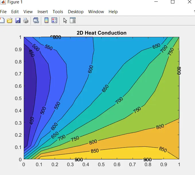
1. This plot shows the temperature gradient across the domain. The values of the different temperature matrixes are plotted along the x and y axis and the contours are drawn around the similar temperature regions.Hence giving a temperature gradient along the domain.

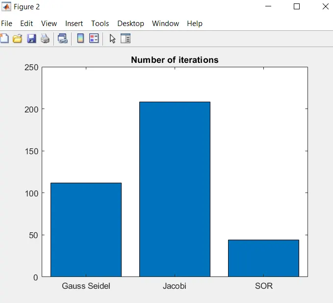
1. This shows the number of iterations as we can see the highest number of iterations is taken by the jacobi method followed by gauss seidel and at last the successive over relaxation method.

2.The Jacobi method takes the highest number of iterations as the values are calculated using old values and once the values are found they are not updated in the same iteration.

3.The gauss seidel takes the 2nd highest number of iterations as the values are calculated using old values and once the values of previous points are found they are updated for finding values at the next point.

4.The sor method takes least as there is a multiplication factor (alpha) that drastically reduces the time. But care should be taken to decide the multiplication factor as lower values can lead to increased time and higher values can lead to overshooting which also leads to increase time.