Week 7 - Simulation of a 1D Super-sonic nozzle flow simulation using Macormack Method
Introduction
We are required to simulate an isentropic flow through a convergent divergent nozzle. Both the conservative and non conservative form of the governing equation is solved using the MacCormack's technique.
Theory
The flow through a nozzle that has a gradual decrease and increase in area is reversible, meaning the flow is isentropic. Hence the flow properties can be found analytically using isentropic flow equations.
`p/p_o=(1+(gamma-1)/2M^2)^(-gamma/(gamma-1))`
`rho/rho_o=(1+(gamma-1)/2M^2)^(-1/(gamma-1))`
`T/T_o=(1+(gamma-1)/2M^2)^-1`
In order to apply a CFD technique we choose the problem with known analytical solution. We setup a CFD solution using MaCCORMACK technique.
Governing Flow Equation
The flow we consider is a quasi 1D flow. It means that the flow properties are a function of only x. It is termed as a quasi flow because the reality of the flow is that the flow properties vary in both x and y direction. Since we assume a quasi flow the physics of the problem is twisted and as a result we will have to form governing equations that satisfies this quasi 1D flow
1. Continuity Equation
Rate of decrease of mass in the control volume=Mass exiting out of the control surface
The integral form
`del/(delt)int int intrho dV+int int rho V.ds=0 `-->(1)
`del/(delt)int int intrho dV=del/(delt)(rho A dx)`-->(2)
`int int rho V.dS=-rhoVA+(rho+drho)(V+dv)(A+dA)`-->(3)
After simplification
`int int rho V.dS=rhoVdA+rhoAdV+AVdrho=d(rhoAV)`-->(4)
Substitute (4) and (2) in (1) and divide by dx we get
`(del(rhoA))/(delt)+(del(rhoAV))/(delt)=0`-->(5)
Conservative form of continuity equation
2.Momentum Equation
F=ma
`del/(delt)int int int(rhou) dV+int int (rho uV).ds=-int int(rho.dS)`-->(1)
`del/(delt)int int int(rhou) dV=del/(delt)(rhoVAdx)`-->(2)
`int int(rhouV).dS=-rhoV^2A+(rho+drho)(V+drV)^2(A+dA)`-->(3)
`int intp.dS=-pA+(p+dp)(A+dA)-2p((dA)/2)`-->(4)
Substituting (2),(3),(4) in (1) we get
`del/(delt)(rhoVAdx)+d(rhoV^2A)=-Adp`-->(5)
Dividing (5) by dx we get
`del/(delt)(rhoVA)+(del(rhoV^2A))/(delx)=-A(delp)/(delx)`-->(6)
Conservative form of momentum equation
3.Energy Equation
`del/(delt)int int intrho (e+V^2/2)dV+int int rho (e+V^2/2)V.ds=int int(pV).dS`-->(1)
`del/(delt)int int intrho (e+V^2/2)dV=del/(delt)rho(e+V^2/2)Adx`-->(2)
`int int rho (e+V^2/2)V.ds=-rho(e+V^2/2)VA+(rho+drho)(e+de)+(V+dV)^2/2(V+dv)(A+dA)`-->(3)
`int intp.dS=-pVA+(p+dp)(V+dV)(A+dA)-2(pV(dA)/2)`-->(4)
Substitute (4),(3),(2) in (1) and simplify.ALso divide by dx
`(del[rho(e+V^2/2)A)]/(delt)+(del[rho(e+V^2/2)VA])/(delx)=-(del(pAV))/(delx)`-->(5)
Conservative form of energy equation
Conservative Form
1.Continuity Equation
`(del(rhoA))/(delt)+(del(rhoAV))/(delt)=0`
2.Momentum Equation
`del/(delt)(rhoVA)+(del(rhoV^2A))/(delx)=-A(delp)/(delx)`
3.Energy Equation
`(del[rho(e+V^2/2)A)]/(delt)+(del[rho(e+V^2/2)VA])/(delx)=-(del(pAV))/(delx)`
Non Conservative Form
1.Continuity Equation
`(del(rhoA))/(delt)+rhoA(delV)/(delx)+rhoV(delA)/(delx)+VA(delrho)/(delx)=0`
2.Momentum Equation
`rho(delV)/(delt)+rhoV(delV)/(delx)=-R(rho(delT)/(delx)+T(delrho)/(delx))`
3.Energy Equation
`rhoc_v(delT)/(delt)+rhoVc_v(delT)/(delx)=-rhoRT[(delV)/(delx)+V(del(lnA))/(delx)]`
We can try advancing and setting up the numerical solution but the flow variables are often referenced to their reservoir values (non dimensional values) .This gives an added asthetic advantage as the values are between 0 to 1.
`T'=T/T_0`
`rho'=rho/rho_0`
`x'=x/L`
`a_0=sqrt(gammaRT_0)`
`V'=V/a_0`
`t'=t/(L/a_0)`
`A'=A/A^ast`
Introducing the non dimensional variables to the non conservative equation and simplifying we get
NON CONSERVATION FORM
Step1: Governing FLow Equations
Continuity Equation
`(delrho')/(delt)=-rho'(delV')/(delx')-rho'V'(del(lnA'))/(delx')+V'(delrho')/(delx')`
Momentum Equation
`(delV')/(delt')=-V'(delV')/(delx')-(1/gamma)((delT')/(delx')+(T')/(rho')(delrho')/(delx'))`
Energy Equation
`(delT')/(delt')=-V'(delT')/(delx')-(gamma-1)T'[(delV')/(delx')+V'(del(lnA'))/(delx')]`
Let us first solve for the flow field variables in the non conservative form and then compare them with the conservative form
Step 2: Finite Difference Equation
1.Grid points
We first divide the entire nozzle using grid points from 1 to N points having an equal distance of dx. In this case we take the grid points (N) to be 31.
2.Maccormack Technique
The Maccormack technique is a predictor corrector technique. i.e we will have to predict the value of a flow field variable and then correct it.
Predicter Step
i) Using taylor series we obtain a formula for finding the predicted values
`barrho_i^(t+trianglet)=rho_i^t+((delrho)/(delt))_i^t(trianglet)`
`barV_i^(t+trianglet)=V_i^t+((delV)/(delt))_i^t(trianglet)`
`barT_i^(t+trianglet)=T_i^t+((delT)/(delt))_i^t(trianglet)`
ii)Then by numerical differencing (forward differencing)we find the values of `del/(delt)` values
`(del rho)/(delt)=-rho_i^t(V_(i+1)^t-V_i^t)/dx-rho_i^tV_i^t(lnA_i+1-lnA_i)/dx-V_i^t(rho_(i+1)^t-rho_i^t)/dx`
`(del V)/(delt)=-V_i^t(V_(i+1)^t-V_i^t)/dx-(1/gamma)[(T(i+1)-T_i)/dx+(T_i^t/rho_i^t)(rho_(i+1)^t-rho_i^t)/dx]`
`(del T)/(delt)=-V_i^t(T_(i+1)^t-T_i^t)/dx-(gamma-1)T_i^t(V_(i+1)-V_i)/dx-V_i^t(lnA_(i+1)^t-lnA_i^t)/dx`
iii)Substitute all the above values in the taylor series formula to find the predicted flow variables
Corrector Step
i)Substitue all the above predicted flow field variables in the corrector step. The corrector step uses rear ward differencing to find the corrected values of `del/(delt)` values
`((del barrho)/(delt))_i^(t+trianglet)=-barrho_i^(t+trianglet)(barV_(i)^(t+trianglet)-barV_(i-1)^t)/dx-barrho_i^(t+trianglet)barV_i^(t+trianglet)(lnA_i+1-lnA_i)/dx-barV_i^(t+trianglet)(barrho_(i+1)^(t+trianglet)-barrho_i^(t+trianglet))/dx`
`((delbar V)/(delt))_i^(t+trianglet)=-barV_i^t(barV_(i)^(t+trianglet)-barV_(i-1)^(t+triangle t))/dx-(1/gamma)[(barT_(i)-barT_(i-1))/dx+(barT_i^(t+trianglet)/barrho_i^(t+trianglet))(barrho_(i)^(t+trianglet)-barrho_(i-1)^(t+trianglet))/dx]`
`((del barT)/(delt))_i^(t+trianglet)=-barV_i^(t+trianglet)(barT_(i+1)^(t+trianglet)-barT_i^(t+trianglet))/dx-(gamma-1)T_i^(t+trianglet)(barV_(i)^(t_triangle)-barV_(i-1)^(t+trianglet))/dx+barV_i^(t+trianglet)(lnA_(i+1)-lnA_i)/dx`
Average Value
The average value is then calculated
`((delrho)/(delt))_(av)=0.5(((delrho)/(delt))+((delbarrho)/(delt)))`
`((delT)/(delt))_(av)=0.5(((delT)/(delt))+((delbarT)/(delt)))`
`((delV)/(delt))_(av)=0.5(((delV)/(delt))+((delbarV)/(delt)))`
Corrected Values
`rho_i^(t+trianglet)=rho_i^t+((delrho)/(delt))_(av)(trianglet)`
`V_i^(t+trianglet)=V_i^t+((delV)/(delt))_(av)(trianglet)`
`T_i^(t+trianglet)=T_i^t+((delT)/(delt))_(av)(trianglet)`
Step 3:Time Step
Since the above governing equation is hyberbolic we use the condition C<=1 of the courant number
The formula used to calculate time step is
`triangle t=C[(trianglex)/((T_i)^(1/2)+V_i)]`
We calculate the different time step for each grid point and then take the minimum time step as the required value
dt=0.02
Step 4:Boundary Conditions
We cannot find the values of flow field variables at the boundary condition since numerically differentiating the values at the boundary ,we will have to obtain value from out of the domain. Hnece we require boundary conditions.
The above governing equation is hyperbolic in nature as a result it has two method of characteristics. The propogation of MOC into or away from the domain tells us whether the variable should be fixed or should float.
Inflow
At the subsonic inflow point there are 2 method of characteristic one goes away from the domain and one into the domain. As a result we float the velocity and keep density and time fixed.
The velocity is found in a time step by linear interpolation
slope=(V3-V2)/dx
slope=(V1-V2)/dx
Equate and we get
V1=2V2-V3--> Float
rho=1-->fixed
T=1 --> fixed
Outflow
At the supersonic outflow the 2 MOCs deviate awway from the domain as a result all the flow field variables are made to float at th N point.
V(N)=2V(N-1)-V(N-2)--> Float
rho(N)=2rho(N-1)-rho(N-2)--> Float
T(N)=2T(N-1)-T(N-2)--> Float
Step 5:Initial Condition
To start the process we have to define the initial values of the flow field variables at the grid points @t=0. We will have to carefully consider the initial values because a closer value to the final solution may cause convergence to occur at a faster rate.
Here the initial condition are constructed based on the grid points
`rho=1-0.3146x`
`T=1-0.231x`
`V=(0.1+1.09x)T^(1/2)`
The area is given as a function of x
`A=1+2.2(x-1.5)^2`
CONSERVATIVE FORM
Step 1:Governing Equations
When the above conservative form derived is written in terms of non dimensional flow field variable we get
Continuity Equation
`(del(rho'A'))/(delt)+(del(rho'A'V'))/(delt)`
Momentum Equation
`(del(rho'A'V'))/(delt)+(del(rho'A'V'^2+(1/gamma)p'A'))/(dx')=(1/gamma)p'(delA')/(dx')`
Energy Equation
`(del(rho'((e')/(gamma-1)+(gamma/2)V'^2)A'))/(delt')+(del(rho'((e')/(gamma-1)+(gamma/2)V'^2)V'A'+p'A'V'))/(delx')=0`
The above equations are simplified by writing in terms of vectors. [U1 U2 U3] solution vector,[F1 F2 F3] Flux Vector ,[J1] Source vector
`U1=rho'A'`
`U2=rho'A'V'`
`U3=rho'((e')/(gamma-1)+(gamma/2)V'^2)A'`
`F1=rho'A'V'`
`F2=rho'A'V'^2+(1/gamma)p'A'`
`F3=rho'((e')/(gamma-1)+(gamma/2)V'^2)V'A'+p'A'V'`
`J2=(1/gamma)p'(delA')/(delx'`
Writing in terms of simplified vectors
`(delU1)/(delt')=-(delF1)/(delx')`
`(delU2)/(delt')=-(delF2)/(delx')+J2`
`(delU3)/(delt')=-(delF3)/(delx')`
Decoding of Flow variables
When we solve the above governing equation we get the value for the solution,flux and souce terms and not the original flow field variables.Hence we have to decode the solution to the flow field variables.
`rho'=(U1)/(A')`
`V'=(U2)/(U1)`
`T'=(gamma-1)((U3)/(U1)-(gamma/2)V'^2)`
`p'=rho'T'`
Pure Form
To obtain purity in the governing equation the right hand side of the equation is written in terms of U1,U2,U3
F1=F1(U1,U2,U3)
F2=F2(U1,U2,U3)
F3=F3(U1,U2,U3)
J2=J(U1,U2,U3)
All the flow field variables in F1,F2,F3 and J are written in terms of U1,U2,U3 from the above decoding of source vectors to the field variables as a result we get
F1=U2
`F2=U_2^2/U_1+(gamma-1)/gamma[U_3/U_1-(gamma)/2U_2^2/U_1]`
`F_3=(gammaU_2U_3)/U_1-(gamma(gamma-1))/2(U_2^2/U_1^2)`
`J_2=(gamma-1)/gamma(U_3-gamma/2(U_2^2/U_1))(del(lnA))/(delx)`
The purity is followed because solving F1,F2,F3 and J in terms of variables(primitive) leads to instabilities
Step 2:Boundary Conditions
As in the case of non conservative form the number of variables to float and to be fixed is same both on the inflow and ouflow side. But here as the governing equation deals with the solving of source terms instead of primitive variables ,the boundary conditions are given for U1,U2,U3.
The equations to solve U1,U2,U3 at the boundaries is given by the decoding of source terms except that the source term are know the unknown and the primitive variables are known.
Inflow
`U_1(1)=(rho'A')_(i=1)=A'_(i=1)` as pho=1
`U_2(i=1)=2U_(2(i=2))-U_(2(i=3))`
`U_3=rho'((e')/(gamma-1)+(gamma/2)V'^2)A'` e' can be replaced with T' as `e'=e/e_0=(c_vT)/(c_vT_0)=T/T_0=T'`
Outflow
`(U_1)_N=2(U1)_(N-1)-(U_1)_(N-2)`
`(U_2)_N=2(U_2)_(N-1)-(U_2)_(N-2)`
`(U_3)_N=2(U3)_(N-1)-(U_3)_(N-2)`
Step 3:Inital Condition
Since we solve for the solution vector terms we require the values of U terms at t=0. But the U terms can only be found out by the flow field variables. Hence we find the initial conditions for rho,T,V at t=0.
for 0<=x'<=0.5
`rho'=1`
`T'=1`
for 0.5<=x'<=1.5
`rho'=1-0.366(x'-0.5)`
`T'=1-0.167(x'-0.5)`
for 1.5<=x'<=3.5
`rho'=0.634-0.3879(x'-1.5)`
`T'=0.833-0.3507(x'-1.5)`
The reason we employ a fine assumption of initial values for the conservative form is because it is very sensitive.
Using the above assumed inital values of variables and the fact that one of the dependent variable is physically mass flow rate as a result we can assume a constant mass flow rate at t=0 and calculate V'
`V'=U_2/(rho'A')`
Then we find the initial values of dependent variable(U) by substituting the above initial values of primitive variables in the below equation at all the grid points
`U1=rho'A'`
`U2=rho'A'V'`
`U_3=rho'((e')/(gamma-1)+(gamma/2)V'^2)A'`
Step 4:Finite Difference
In this step we numerically differentiate the governing equaiton using the Maccormack's technique similar to the non conservative part
Predictor Step
i)We calculate the predicted value of U1,U2,U3 for the next time step from the equation obtained from the taylor series.
ii)The predicted `(delU_1)/(delT),(delU_2)/(delT),(delU_3)/(delT)` is obtained by the forward differencing the governing equation which involves the flux and source term of the current time step
iii)The values are then put into the taylor series to obtain predicted value of U1,U2,U3.
iv)Using U1,U2,U3 the predicted values of flow variables are decoded.
v)Then using the flow variables predicted values of Flux and Source terms fro the next time step are found.
Corrector Step
i)The corrected `(delU_1)/(delT),(delU_2)/(delT),(delU_3)/(delT)` is obtained by backward differncing of the governing equation which invloves the predicted values of flux and source terms.
ii)The average `(delU_1)/(delT),(delU_2)/(delT),(delU_3)/(delT)` is obtained by averaging the value of predicted and corrector values
iii)The corrected [U1,U2,U3]values are found and then the corrected flow field variables are decoded from them.
After following the above steps and iterating the above steps for a 1400 time we get the exact solutions of the flow field variables for both the conservative and non conservative equation. The codes are written in MATLAB
Programming Code
main.m
%Creating the gridpoints
n=31;
x=linspace(0,3,n);
nt=1000;

%Value of dx,dt and gamma
dx=x(2)-x(1);
dt=0.026;
gamma=1.4;
[rho_non,T_non,V_non]=non_conservative(n,x,nt,dx,dt,gamma);
[rho_cons,T_cons,V_cons]=conservative(n,x,nt,dx,dt,gamma);


function[rho,T,V]=non_conservative(n,x,nt,dx,dt,gamma);
%Non Conservation
%Calculating inital value @ t=0 of Density(rho),Temp(T),Area(A) as a function of space
rho=1-0.3146*x;
T=1-0.2314*x;
V=(0.1+1.09*x).*T.^(1/2);
A=1+2.2*(x-1.5).^2;
M=V./sqrt(T);
p=rho.*T;
%Time Step
for k=1:nt

%Values of flow variables at previous time step
rho_old=rho;
T_old=T;
V_old=V;

%Predictor step
 for i=2:n-1
%Forward Space Differencing

del_V=(V(i+1)-V(i))/dx;
del_A=(log(A(i+1))-log(A(i)))/dx;
del_rho=(rho(i+1)-rho(i))/dx;
del_T=(T(i+1)-T(i))/dx;

%Continuity Equation
del_rho_p(i)=-rho(i)*del_V-rho(i)*V(i)*del_A-V(i)*del_rho;
%Momentum Equation
del_V_p(i)=-V(i)*del_V-(1/gamma)*(del_T+(T/rho)*(del_rho));
%Energy Equation
del_T_p(i)=-V(i)*(del_T)-(gamma-1)*(T(i))*(del_V+V(i)*del_A);

%Update
rho(i)=rho(i)+(del_rho_p(i))*dt;
V(i)=V(i)+(del_V_p(i))*dt;
T(i)=T(i)+(del_T_p(i))*dt;
end

%corrector step
for i=2:n-1
%Backward Space Differencing
del_V=(V(i)-V(i-1))/dx;
del_A=(log(A(i))-log(A(i-1)))/dx;
del_rho=(rho(i)-rho(i-1))/dx;
del_T=(T(i)-T(i-1))/dx;

%Continuity Equation
del_rho_c(i)=-rho(i)*del_V-rho(i)*V(i)*del_A-V(i)*del_rho;
%Momentum Equation
del_V_c(i)=-V(i)*del_V-(1/gamma)*(del_T+(T/rho)*(del_rho));
%Energy Equation
del_T_c(i)=-V(i)*(del_T)-(gamma-1)*(T(i))*(del_V+V(i)*del_A);
end

del_rho_av=0.5*(del_rho_c+del_rho_p);
del_V_av=0.5*(del_V_c+del_V_p);
del_T_av=0.5*(del_T_c+del_T_p);

%Corrected Values
for i=2:n-1
rho(i)=rho_old(i)+(del_rho_av(i))*dt;
V(i)=V_old(i)+(del_V_av(i))*dt;
T(i)=T_old(i)+(del_T_av(i))*dt;

end
T_index(k)=T(16);
V_index(k)=V(16);
rho_index(k)=rho(16);

%boundary conditions
V(1)=2*V(2)-V(3);
V(n)=2*V(n-1)-V(n-2);
T(n)=2*T(n-1)-T(n-2);
rho(n)=2*rho(n-1)-rho(n-2);

for i=1:n
M(i)=V(i)/sqrt(T(i));
p(i)=rho(i)*T(i);
end
M_index(k)=M(16);
p_index(k)=p(16);

if(k==1 || k==100 || k==200 || k==300 || k==700)
    for i=1 :n
        massflow(i)=rho(i)*A(i)*V(i);
        mass_index(i,j)=massflow(i);

    end
    j=j+1;

end

end
k=1:nt;
figure(1)
subplot(5,1,1);
plot(x,V);
xlabel('x');
ylabel('Velocity');
subplot(5,1,2)
plot(x,T);
xlabel('x');
ylabel('Temperature');
subplot(5,1,3);
plot(x,rho);
xlabel('x');
ylabel('Density');
subplot(5,1,4);
plot(x,p);
xlabel('x');
ylabel('pressure');
subplot(5,1,5);
plot(x,M);
xlabel('x');
ylabel('Mach Number');
suptitle({'Non Conservative Form','Variation of flow parameters along x direction'});
figure(2)
subplot(5,1,1);
plot(k,T_index);
xlabel('Time Step');
ylabel('Temperature');
subplot(5,1,2);
plot(k,V_index);
xlabel('Time Step');
ylabel('Velocity');
subplot(5,1,3);
plot(k,rho_index);
xlabel('TIme Step');
ylabel('Density');
subplot(5,1,4)
plot(k,p_index);
xlabel('Time Step');
ylabel('pressure');
subplot(5,1,5)
plot(k,M_index);
xlabel('Time Step');
ylabel('Mach Number');
suptitle({'Non Conservative Form','Convergence of flow parameters'});
figure(5)
plot(x,mass_index);
xlabel('x/L');
ylabel('Non Dimensional Mass Flow Rate');
legend('0dt','100dt','200dt','300dt','700dt');
title('Mass FLow Rate');

end


function[rho,T,V]=conservative(n,x,nt,dx,dt,gamma)

%initial values
A=1+2.2*(x-1.5).^2;

for i= 1 : n
    if(x(i) >=0 && x(i)<0.5)
    rho(i)=1;
    T(i)=1;
    end

    if(x(i)>=0.5 && x(i)<1.5)
    rho(i)=1-0.366*(x(i)-0.5);
    T(i)=1-0.167*(x(i)-0.5);
    end

    if(x(i)>=1.5 && x(i)<=3.5)
    rho(i)=0.634-0.3879*(x(i)-1.5);
    T(i)=0.833-0.3507*(x(i)-1.5);
    end

end


    for i=1:n
    V(i)=0.59/(rho(i)*A(i));

    U1(i)=rho(i)*A(i);
    U2(i)=rho(i)*A(i)*V(i);
    U3(i)=rho(i)*((T(i)/(gamma-1))+(gamma/2)*V(i)^2)*A(i);

    F1(i)=U2(i);
    F2(i)=(U2(i)^2/U1(i))+(gamma-1)/(gamma)*(U3(i)-(gamma/2)*(U2(i)^2/U1(i)));
    F3(i)=gamma*((U3(i)*U2(i))/U1(i))-(gamma*(gamma-1)/2)*(U2(i)^3/U1(i)^2);
    end


%time loop
for k=1:nt
%predictor step
    U1_old=U1;
    U2_old=U2;
    U3_old=U3;

    for i=1:n
    F1(i)=U2(i);
    F2(i)=(U2(i)^2/U1(i))+((gamma-1)/(gamma))*(U3(i)-(gamma/2)*(U2(i)^2/U1(i)));
    F3(i)=(gamma*((U3(i)*U2(i))/U1(i)))-((gamma*(gamma-1))/2)*(U2(i)^3/U1(i)^2);

    end

    for i=2:n-1
        J2(i)=(1/gamma)*rho(i)*T(i)*((A(i+1)-A(i))/dx);
    end

    for i=2:n-1

    delU1_p(i)=(-(F1(i+1)-F1(i))/dx);
    delU2_p(i)=(-(F2(i+1)-F2(i))/dx)+ J2(i);
    delU3_p(i)=(-(F3(i+1)-F3(i))/dx);

     %predictor values of dependent variables
    U1(i)=U1(i)+(delU1_p(i)*dt);
    U2(i)=U2(i)+(delU2_p(i)*dt);
    U3(i)=U3(i)+(delU3_p(i)*dt);

    %decoding of flow variables by predictor variables
    rho(i)=U1(i)/A(i);
    T(i)=(gamma-1)*(U3(i)/U1(i)-(gamma/2)*(U2(i)/U1(i)));
    end

   %predictor values of Flux vector
    for i=2:n-1
    F1(i)=U2(i);
    F2(i)=(U2(i)^2/U1(i))+((gamma-1)/(gamma))*(U3(i)-(gamma/2)*(U2(i)^2/U1(i)));
    F3(i)=(gamma*((U3(i)*U2(i))/U1(i)))-(((gamma*(gamma-1))/2)*(U2(i)^3/U1(i)^2));
    J2(i)=(1/gamma)*rho(i)*T(i)*((A(i)-A(i-1))/dx);
    end

    %corrector method
    for i=2:n-1
    delU1_c(i)=-(F1(i)-F1(i-1))/dx;
    delU2_c(i)=-(F2(i)-F2(i-1))/dx+J2(i);
    delU3_c(i)=-(F3(i)-F3(i-1))/dx;
    end

    delU1_av=0.5*(delU1_p+delU1_c);
    delU2_av=0.5*(delU2_p+delU2_c);
    delU3_av=0.5*(delU3_p+delU3_c);

    for i=2:n-1
    U1(i)=U1_old(i)+(delU1_av(i)*dt);
    U2(i)=U2_old(i)+(delU2_av(i)*dt);
    U3(i)=U3_old(i)+(delU3_av(i)*dt);
    end

    %inflow BC
    U1(1)=A(1);
    U2(1)=2*U2(2)-U2(3);
    U3(1)=U1(1)*((1/(gamma-1))+(gamma/2)*V(1)^2);

    %outflow BC
    U1(n)=2*U1(n-1)-U1(n-2);
    U2(n)=2*U2(n-1)-U2(n-2);
    U3(n)=2*U3(n-1)-U3(n-2);

    for i=1:n
    rho(i)=U1(i)/A(i);
    T(i)=(gamma-1)*(U3(i)/U1(i)-(gamma/2)*(U2(i)/U1(i)));
    V(i)=0.59/(rho(i)*A(i));
    M(i)=V(i)/sqrt(T(i));
    p(i)=rho(i)*T(i);
    end

    T_index(k)=T(16);
    V_index(k)=V(16);
    rho_index(k)=rho(16);
    M_index(k)=M(16);
    p_index(k)=p(16);


 if(k==1 || k==100 || k==200 || k==300 || k==700)
    for i=1 :n
        massflow(i)=rho(i)*A(i)*V(i);
        mass_index(i,j)=massflow(i);

    end
    j=j+1;


end
end

k=1:nt;
figure(3)
subplot(5,1,1);
plot(x,V);
xlabel('x');
ylabel('Velocity');
subplot(5,1,2)
plot(x,T);
xlabel('x');
ylabel('Temperature');
subplot(5,1,3);
plot(x,rho);
xlabel('x');
ylabel('Density');
subplot(5,1,4);
plot(x,p);
xlabel('x');
ylabel('pressure');
subplot(5,1,5);
plot(x,M);
xlabel('x');
ylabel('Mach Number');
suptitle({'Conservative Form','Variation of flow parameters along x direction'});
figure(4)
subplot(5,1,1);
plot(k,T_index);
xlabel('Time Step');
ylabel('Temperature');
subplot(5,1,2);
plot(k,V_index);
xlabel('Time Step');
ylabel('Velocity');
subplot(5,1,3);
plot(k,rho_index);
xlabel('x');
ylabel('Density');
subplot(5,1,4)
plot(k,p_index);
xlabel('Time Step');
ylabel('pressure');
subplot(5,1,5)
plot(k,M_index);
xlabel('Time Step');
ylabel('Mach Number');
suptitle({'Conservative Form','Convergence of flow parameters'});
figure(6)
plot(x,mass_index);
xlabel('x/L');
ylabel('Non Dimensional Mass Flow Rate');
legend('0dt','100dt','200dt','300dt','700dt');
title('Mass FLow Rate');
end
Grid Independence
The flow parameters that we get is a function of number of grid points. If we increase the number of grid points the mesh becomes finer and the values change. Grid independence shows us whether the solution varies if we increase or decrease the number of grid points.
For example when the number of grid points is 31 we get T/T0 as 0.836 and when we double the grid points to 62 we get T/T0 as 0.835. The change in value is really small as a result we can say that with n=31 grid independence is reached.
Grid Independence depends on whether we can tolerate less accurate results with shorter convergence time or we would really want a highly accurate result with increase in space and time consumption.
Plots
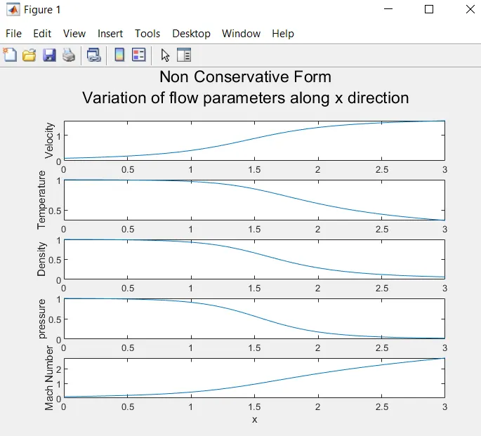
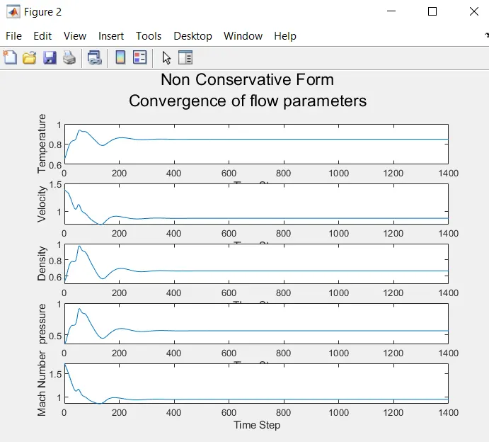
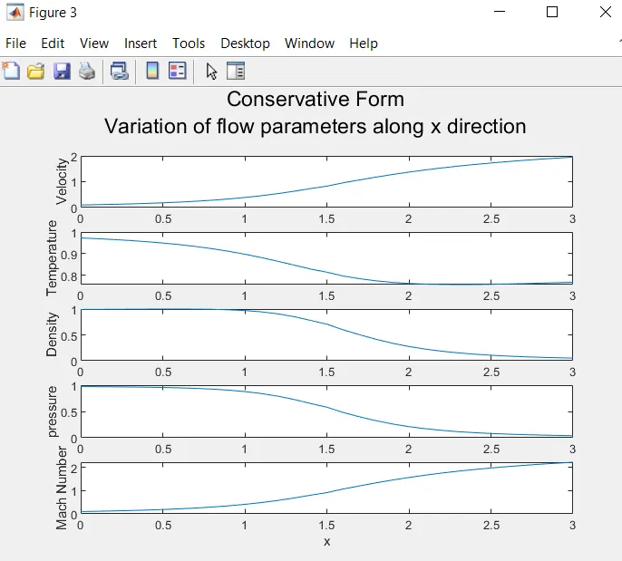
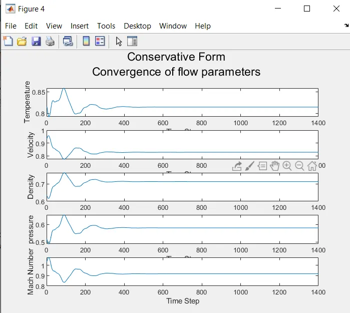
Inference
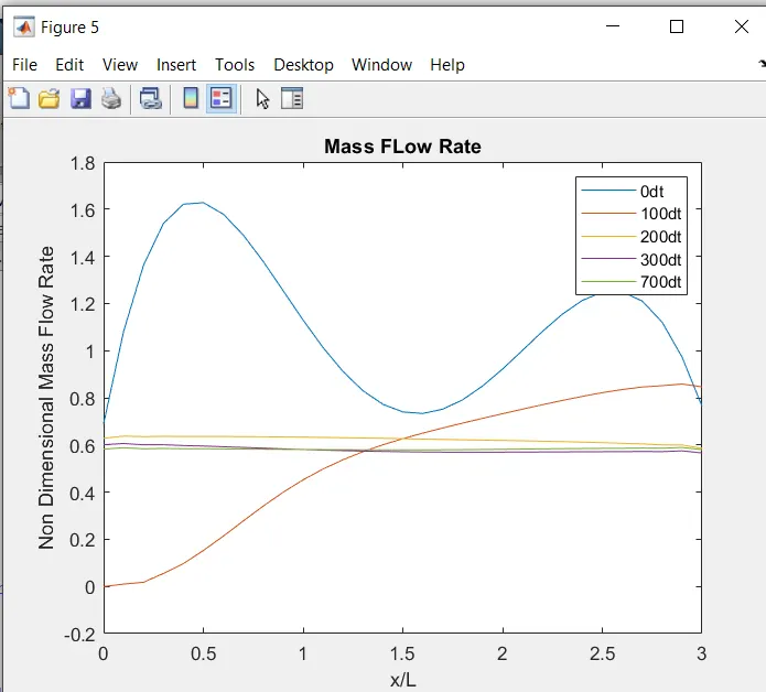
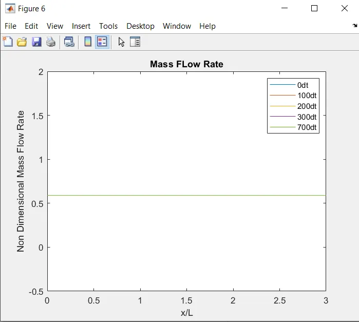
1.The conservation form yields a better mass distribution as seen from the last two plots.The non conservation form constant mass flow is acheived only at a later time step whereas in the conservation form mass flow is acheived from the very begining. The reason behind this is because mass flow rate is a primary dependent variable in the conservation form. Whereas in the non conservation form it is calculated as a secondary from primary flow parameters.
2.The calculation effort for the conservation form is a bit higher than the non conservation form due to the addition of source,flux and solution vectors.
3. The convergence of flow parameters plot gives us an idea of how fast the convergence occurs.We can infer from the graph that about 800 iterations is enougn for the convergence to reach.
4.The non conservation form gives a higher accuracy as compared to the conservation form.
Conclusion
We can not say that one form is better than the other. It depends on wether you want the flux variables to be accurate or the primitve ones.If its flux variables then we will have to go with conservative form if not non conservative is the best case.