Week 4.2: Project - Transient simulation of flow over a throttle body
Aim:
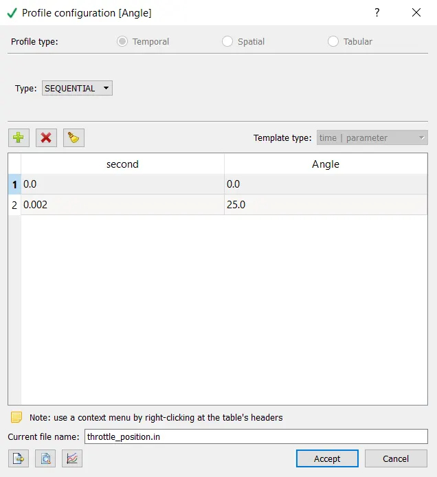
In this project we run a transient simulation of air over a throttle body using converge cfd and post process the results. The throttle body is at `0^o`the beginning of the simualtion and is rotated to about `25^o` till the end of simulation.
Theory:
A throttle is used to control the amount of fluid flowing.The throttle in open position allows the full passage of fluid whereas a throttle in closed position is used to constrict the flow of fluid . The throttle valve can be rotated at various angle depending on the amount of fluid to flow through.
Throttles are primarly used to control the amount of power by regulating the amount of fluid passage eg:Turbines,ICE
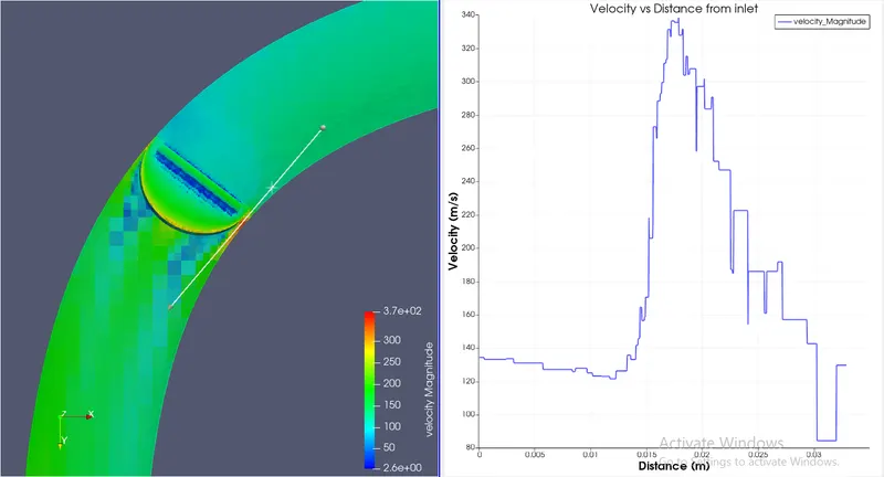
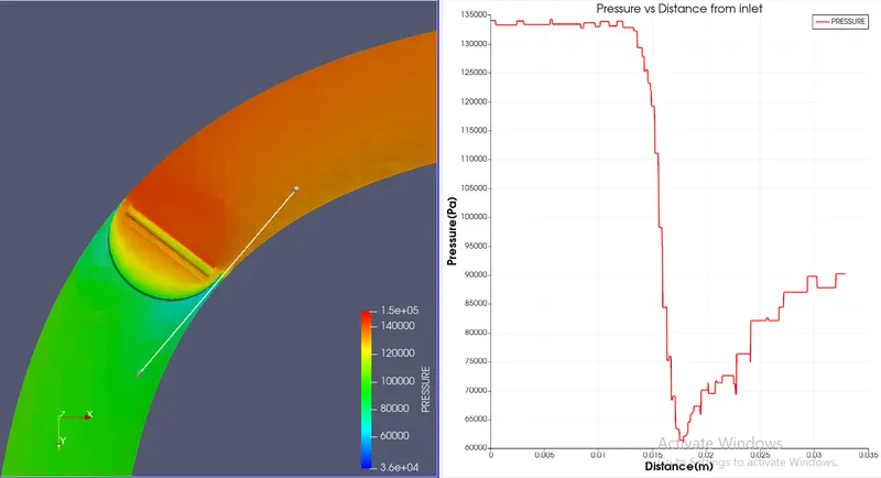
In a flow over a throttle , area near the sides of the walls get reduced due to the inclination of the throttle at an angle .In order to satisfy the conservation of mass when the area is reduced the same amount of fluid has to pass through the reduced area as a result there is an increase in velocity of the fluid whcih results in decrease in pressure with accordance to bernoulli's equation.

1. Geometry:
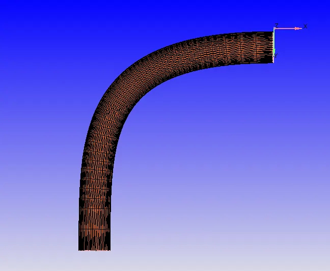
The geometry is imported as a .stl file into converge.
1.1 Boundary Flagging
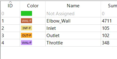
The required boundaries are flagged
Case Setup:
1. Materials
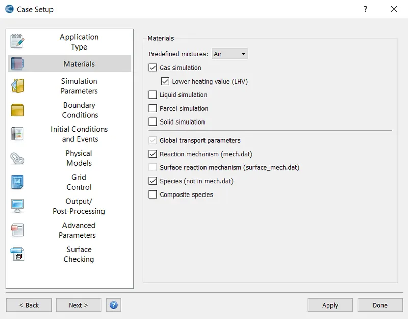
The predefined mixture is selected to be air.
2. Simulation Parameters
2.1. Run Parameters
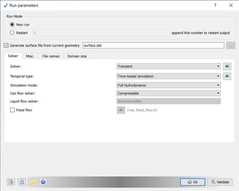
The solver type is chosen as transient and simulation mode is full hydrodynamic
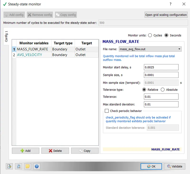
2.2 Steady State Monitor
The mass flow rate and average velocity at outlet is monitored for convergence
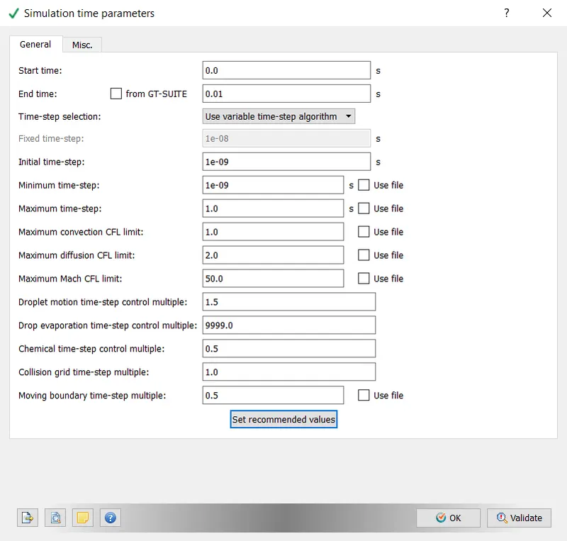
2.3 Simlulation Time Parameter
Since it is a transient simulation, time is taken in seconds.
the end time is calculated as follows:
In steady state analysis the inlet average velocity was 80 m/s.The characteristic length of the model is 0.11 m.Therefore the time for the flow to travel the pipe once is `0.11/80=``0.025s`.
We would want to simulate it for 5 times the time taken which gives us 10 ms or 0.01s .
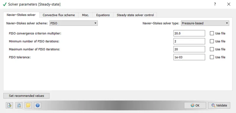
2.4 Solver Parameters
Solver type is chosen to be pressure based
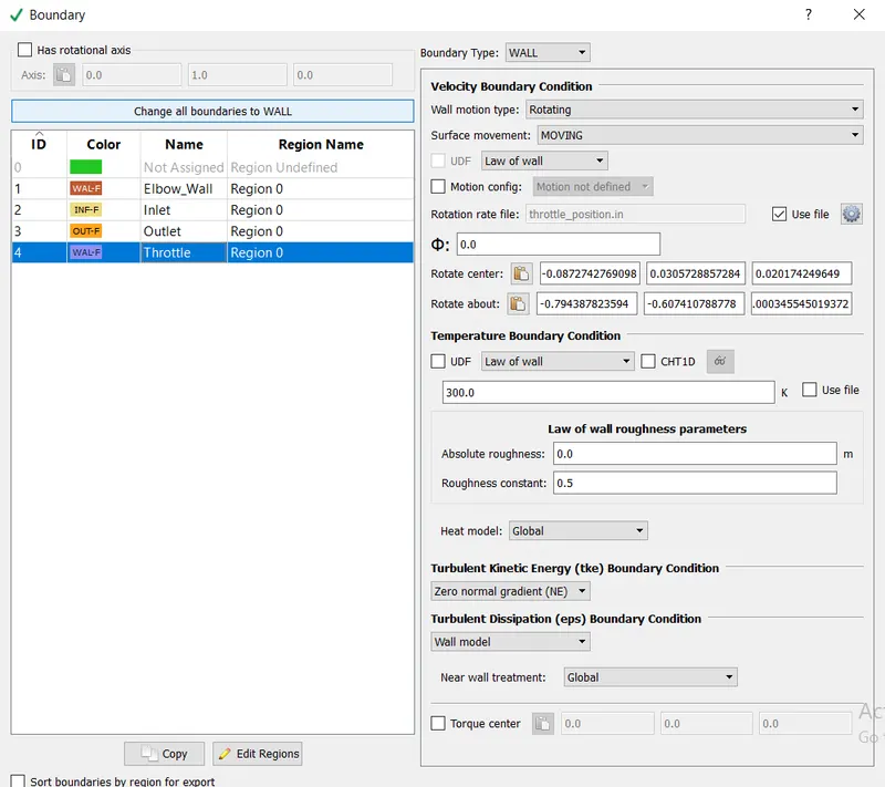
3. Boundary Conditions
The boundary conditions for the different boundaries Inlet , Oulet,Elbow wall & Throttle are given. Inlet and outlet pressure are specified and the throttle's surface movement is taken as moving , type rotating.
The rotation center and rotation axis of the throttle is given as inputs.
For the rotation a rate an .in file is given as input.
4. Regions and Initialization
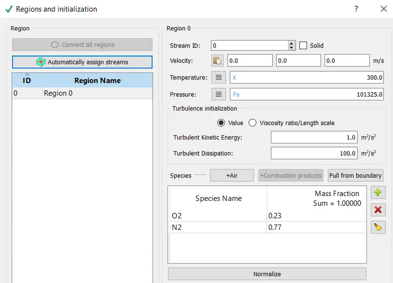
The region is defined containing mixture of air and inital values of pressure and temperatures are specified
5.Physical Model
The turbulence model of RANS_K_EPS_RNG is used
6.Grid Control
6.1 Base Grid
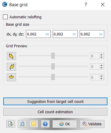
A size of 2mm is used as a base grid
6.2 Fixed embedding
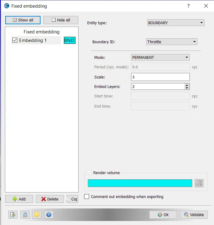
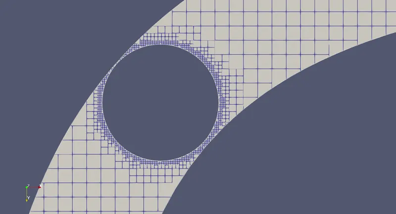
Around the throttle boundary a embedding of scale 3 is used.
Scale defines the level of refinement for embedding. Represents the value of n in dx_base/2^n.
Ouptut Files
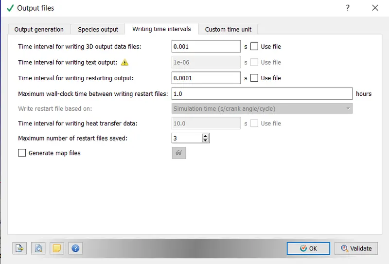
The time interval for writting 3d,text ouput and restart files are mentioned in seconds.
Post Processing
The post processing of results is done using paraview package.
Grid
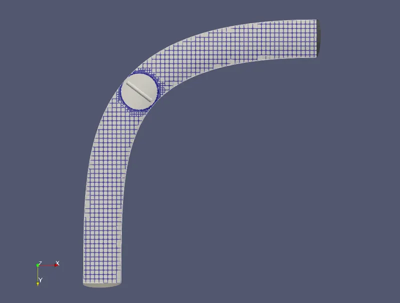
At `0^o`
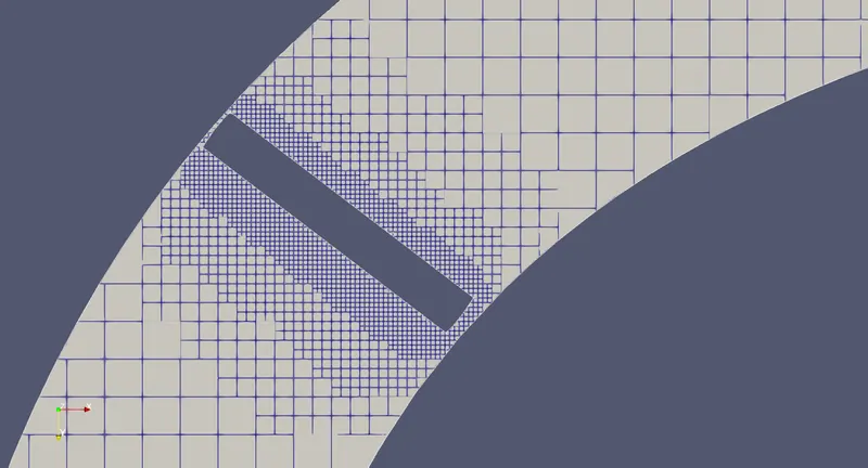
At `25^o`
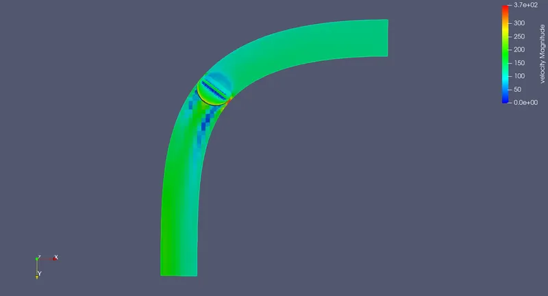
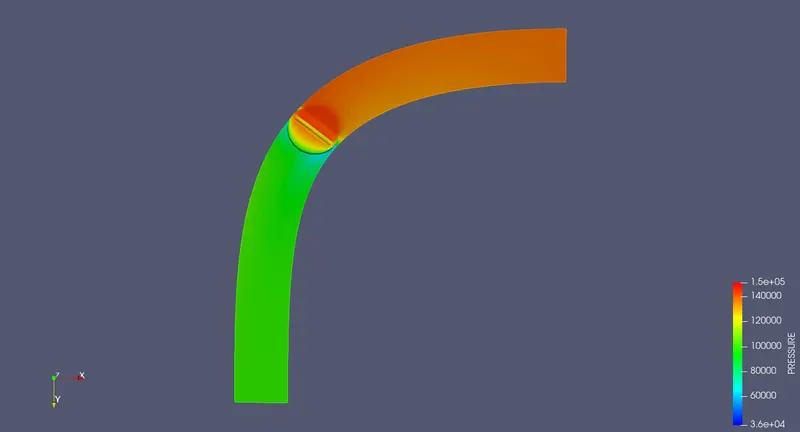
The results are shown when the throttle is @ `25^o`.
Velocity Contour
Pressure Distribution
Converge Plots
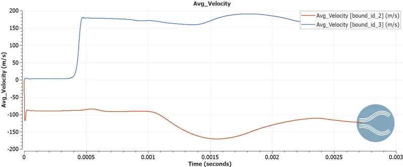
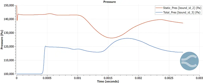
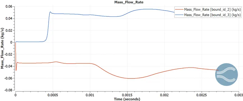
bound_id_2=inlet
bound_id_3=oultlet
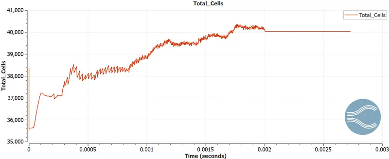
1. Total cell count
2. Average Velocity
3. Pressure
4. Mass Flow Rate
Flow Simulation
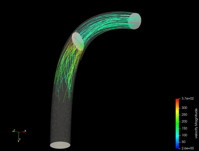
Observations:
1.The embedding scale set to 3 is evidently shown in the grid image as the grids around the throttle is refined as compared to the base grid.We can also notice that the embedding changes with the change in the throttle position.
2.The flow of fluid is hindered due to the throttle being rotated at an angle of 25 degree as a result the velocity of flow decreases upstream which results in the increase in pressure as can be seen in the velocity and pressure contour.
2.As we can see in the plots for both velocity contour and pressure distribution above , the velocity of fluid abruptly increases when it passes thorugh the constriction and in the pressure plot the same region has decrease in pressure with accordance to bernoulli's theorem.
3.We can also observe the places where flow seperation occurs with the presence of low circulation velocity vortices.
4.The cell count keeps on changing with the change in throttle position this can be seen in the cell count plot. It reaches a steady number after the throttle has been turned to 25 degrees after which the throttle is stationary.
5.From the converge plots we can see that the simulation ran for 2.726752754e-03 seconds this is because the monitoring variable of average mass flow and average velocity at oulet reached congvergence @ about 2.726752754e-03 seconds.
converge.log output
MAX CFL= 9.9987e-01, MAX VISCOSITY CFL= 1.2670e-01, MAX CONDUCTION CFL= 1.4135e-01, MAX MASS DIFFUSION CFL= 1.6244e-01, MAX MACH CFL = 2.0765e+00
time-step limit = dt_cfl
Current status of monitored variable MASS_FLOW_RATE@BOUND_ID_3 after 516 iterations: CONVERGED. Tolerance levels (current|target) for mean-diff: 9.98e-03|1.00e-02, for std-deviation: 1.18e-03|1.00e-02
Current status of monitored variable AVG_VELOCITY@BOUND_ID_3 after 516 iterations: CONVERGED. Tolerance levels (current|target) for mean-diff: 9.11e-03|1.00e-02, for std-deviation: 8.76e-04|1.00e-02
All monitored variables have now satisfied the steady-state criteria.
Found file STOP. Finishing job...
6.The other converge plots also seemed to have converged
7.The flow is shown as using the stream tracer.