Week 8 - BlockMesh Drill down challenge
Introduction
We are required to simulate an incompressible-laminar-viscous flow over a backward facing step geometry for two seperate cases one with no grading factor and another with a grading factor of 0.2 using OpenFoam.
Explanation of the simulation and the steps followed
PRE-PROCESSING
1.Determination of Solver
Our first step should be to determine what solver to be used to solve the given simulation. As the problem involves incompressible laminar flow to be solved in a transient state. It is best to go with the icoFoam solver. The path to the solver is cd tutorials/incompressible/icoFoam/.
It is not advised to run the simultioan in the tutorials itself as a result we have got to copy the respective tutorial and paste it in the run directory where we can modify the files and run it. To copy the tutorial enter cp -r icoFoam/ $FOAM_RUN while in the incompressible directory.
2.Modification of geometry and mesh
The next step includes modification of the existing geometry to the given new geometry. For this we will have to go to the blockMeshDict file which is a dictionary file. To path to travel to the file is cd run/cavity/cavity/system/ in the system directory we type gedit blockMeshDict.
In the dictionary file we
1.Edit the vertices to obtain the required geometry.
2.Create blocks to mesh the entire geometry.
3.Name the patches and set the type of it.
blockMeshDict
/*--------------------------------*- C++ -*----------------------------------*\
  =========                 |
  \\      /  F ield         | OpenFOAM: The Open Source CFD Toolbox
   \\    /   O peration     | Website:  https://openfoam.org
    \\  /    A nd           | Version:  8
     \\/     M anipulation  |
\*---------------------------------------------------------------------------*/
FoamFile
{
    version     2.0;
    format      ascii;
    class       dictionary;
    object      blockMeshDict;
}
// * * * * * * * * * * * * * * * * * * * * * * * * * * * * * * * * * * * * * //


convertToMeters 0.001;

vertices
(
    (0 0 0)
    (80 0 0)
    (80 10 0)
    (0 10 0)
    (200 0 0)
    (200 10 0)
    (80 -10 0)
    (200 -10 0)

    (0 0 1)
    (80 0 1)
    (80 10 1)
    (0 10 1)
    (200 0 1)
    (200 10 1)
    (80 -10 1)
    (200 -10 1)
);


blocks
(
    hex (0 1 2 3 8 9 10 11) (200 20 1) simpleGrading (1 1 1)
    hex (1 4 5 2 9 12 13 10) (200 20 1) simpleGrading (1 1 1)
    hex (6 7 4 1 14 15 12 9) (200 20 1) simpleGrading (1 1 1)

);

edges
(
);

patches
(


	 patch inlet

	(

	(0 8 11 3)

        )


    	patch outlet

    	(

    	(4 5 13 12)

    	(4 12 15 7)

    	)


    empty frontAndBack

   (

    (8 9 10 11)

    (9 12 13 10)

    (14 15 12 9)

    (0 3 2 1)

    (1 2 5 4)

    (6 1 4 7)


   )


     wall upperWall

    (

    (10 2 3 11)

    (10 13 5 2)


    )

    wall lowerWall

    (

    (1 6 14 9)

    (8 0 1 9)

    (6 7 15 14)

    )
);
Blocks
Each block is always defined by 8 vertices that is the reason we have hex(0 1 2 3 8 9 10 11), the mesh given here is 200x20x1 it means that in the x direction the mesh size is 200, 20 in the y direction and 1 in the z. Since the simulation is a 2D one it makes no sense to increase the mesh size in the z direction.
Boundary Types
1.The inlet and outlet is predominantly set as patch.
2.The front and back which wont influence the computation is set to as empty.
3.The upper,lower and step walls are set as wall.
Grading Factor
The grading factor tells us about the way in which the meshes are either contracted or stretched or remain the same size.
Gf=size of end cell/size of starting cell
A GF =1 implies that the mesh is same throught.
A GF<1 implies that the the mesh is stretched at the begining and reduces further.
A GF>1 implies that the mesh at the begining is contracted and stretches further away.
The 3 values in the GF changes the size if the mesh in the 3 respective direction (x,y,z).
SOLUTION
3.Set the boundary conditions
Pressure
After setting the boundary types we have to set the boundary conditions for both the pressure and the velocity. Both these files can be found in the 0 folder inside cavity.cd/cavity/0/ and then open the p file using gedit p.
p
/*--------------------------------*- C++ -*----------------------------------*\
  =========                 |
  \\      /  F ield         | OpenFOAM: The Open Source CFD Toolbox
   \\    /   O peration     | Website:  https://openfoam.org
    \\  /    A nd           | Version:  8
     \\/     M anipulation  |
\*---------------------------------------------------------------------------*/
FoamFile
{
    version     2.0;
    format      ascii;
    class       volScalarField;
    object      p;
}
// * * * * * * * * * * * * * * * * * * * * * * * * * * * * * * * * * * * * * //

dimensions      [0 2 -2 0 0 0 0];

internalField   uniform 0;

boundaryField
{
    inlet
    {
        type            zeroGradient;
    }

    outlet
    {
        type            fixedValue;
        value		 uniform 0;
    }

    upperWall
    {
    	type		zeroGradient;
    }

    lowerWall
    {
    	type 		zeroGradient
    }

    frontAndBack
    {
        type            empty;
    }
}

// ************************************************************************* //
Dimensions
The dimensions give us the physical dimensions in terms of SI unt.[kg m s K mol A cd].Since it is [0 2 -2 0 0 0 0] it gives us `m^2s^-2`. Which is the SI unit for kinematic pressure.
Internal Field
The internal field gives us the initial values of pressure and since this is a transient simulation initial value is required.
Boundary FIeld
In the boundary Field we set the boundary values for the given problem
1.The inlet,lowerWall and upperWall are given type zeroGradient.which means that pressure is constant at right angles to the boundary with respect to space.
2.The oulet pressure is taken as 0.
3.The frontAndback boundary is taken as empty.
Velocity
Now we have to set the boundary conditions for the velocity which is located in the same directory as pressure. Type gedit U to edit the code.
U
/*--------------------------------*- C++ -*----------------------------------*\
  =========                 |
  \\      /  F ield         | OpenFOAM: The Open Source CFD Toolbox
   \\    /   O peration     | Website:  https://openfoam.org
    \\  /    A nd           | Version:  8
     \\/     M anipulation  |
\*---------------------------------------------------------------------------*/
FoamFile
{
    version     2.0;
    format      ascii;
    class       volVectorField;
    object      U;
}
// * * * * * * * * * * * * * * * * * * * * * * * * * * * * * * * * * * * * * //

dimensions      [0 1 -1 0 0 0 0];

internalField   uniform (0 0 0);

boundaryField
{
   inlet
    {
        type            fixedValue;
        value           uniform (1 0 0);
    }

    outlet
    {

    	type		zeroGradient;
    }

    upperWall
    {
        type            noSlip;
    }


    lowerWall
    {
        type            noSlip;
    }

    frontAndBack
    {
        type            empty;
    }
}

// ************************************************************************* //
Dimension
The dimension for velocity is m/s which is given by [0 1 -1 0 0 0 0].
Internal Field
The initial condition of velocity is 0 in all 3 directions.
Boundary Field
1. The inlet is given as 1m/s.
2.The outlet is set as type zeroGradient.
3.The upperWall and lowerWall are no slip types meaning the flow of fluid over the walls is 0.
4. The frontAndback is type zero.
4.Set the required time step and end time
The time step and end time can be found in the conrolDict file. The file is int the system directory of the cavity file. Use gedit controlDict to open the file
controlDict
/*--------------------------------*- C++ -*----------------------------------*\
  =========                 |
  \\      /  F ield         | OpenFOAM: The Open Source CFD Toolbox
   \\    /   O peration     | Website:  https://openfoam.org
    \\  /    A nd           | Version:  8
     \\/     M anipulation  |
\*---------------------------------------------------------------------------*/
FoamFile
{
    version     2.0;
    format      ascii;
    class       dictionary;
    location    "system";
    object      controlDict;
}
// * * * * * * * * * * * * * * * * * * * * * * * * * * * * * * * * * * * * * //

application     icoFoam;

startFrom       startTime;

startTime       0;

stopAt          endTime;

endTime         0.6;

deltaT          0.00001;

writeControl    timeStep;

writeInterval   20;

purgeWrite      0;

writeFormat     ascii;

writePrecision  6;

writeCompression off;

timeFormat      general;

timePrecision   6;

runTimeModifiable true;


// ************************************************************************* //
The simulation starts at time 0 and ends at time 0.6. The time step is 0.00001 which is calculated by taking into account the courant number. For convection the formula to find the courant number is `C=u dx/dt` .We will take C=1. dx=L/mesh size (0.08/200=0.0004) . U is the maximum velocity. Substituting all this we find dt to be 0.00001.
5.Run the simulation
In the terminal enter blockMesh. This meshes the given geometry with the required mesh size and after the meshing is complete enter the name of the solver icoFoam to run the simulation.
Once the simulation is finished the same steps are taken for the case 2 simulation.The only exception being that the grading factor is modified from 1 to 0.2 in the y direction.
POST_PROCESSING
Type in paraFoam to open paraView to get the results of the simulation.ParaView is a postprocessing software that helps us to visibly see the simulations results and other details.
Case 1
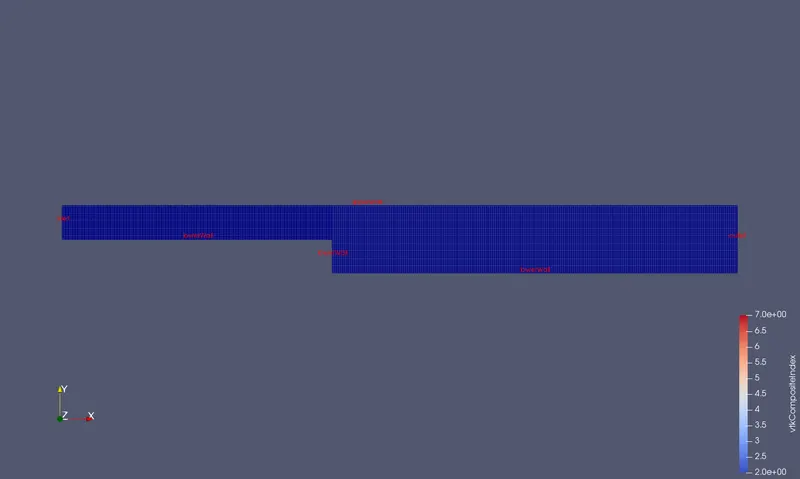
1.Grid
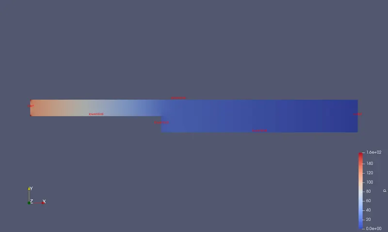
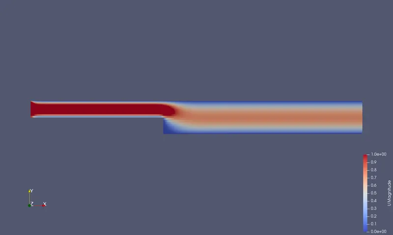
2.Pressure variation at the end time step
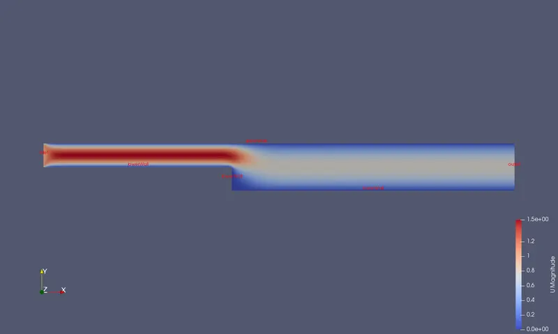
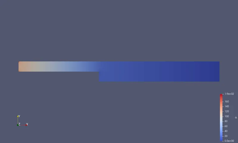
3.Velocity variations at the end time step
Case 2:
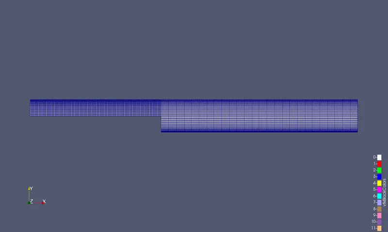
1.Grid
2.Pressure variation
3.Velocity variation
Conclusion
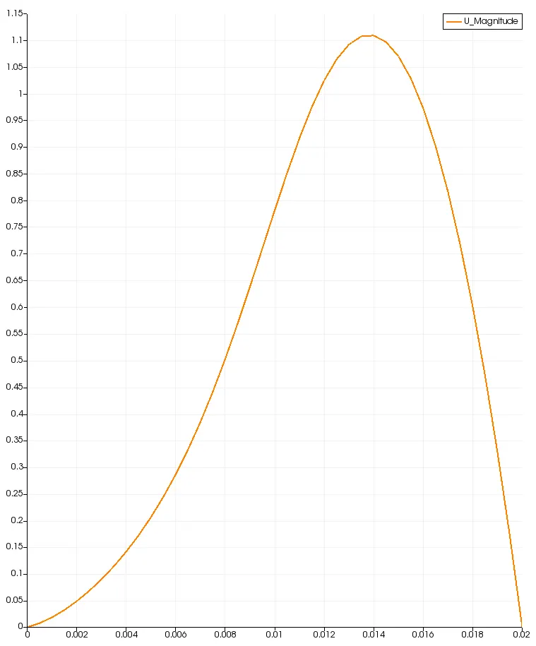
After the simulations for both the cases we can obtain the respective plot of veloicty vs distance by usin plot over line command and set the required direction from the walll i.e 0.085m.
Case1:
Case 2:
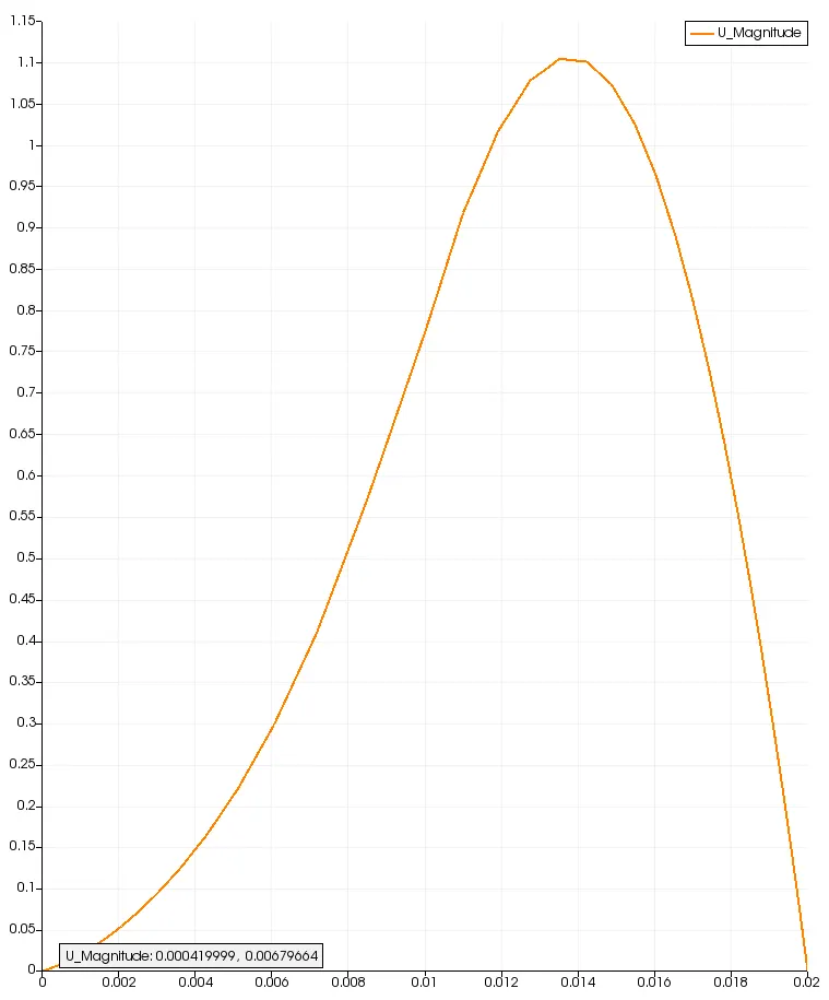
By looking at the velocity plots the changes are not relevant but by assesing the velocity value at that point gives us two different answers for two different cases
Case 1: U=0.64649m/s
Case 2:U=0.637871m/s
Here the importance of grading factor should be stated, the lower the grading factor implies that the finer the mesh becomes, but finer meshes result in increased computational time. Hence finer meshes must be used in boundaries to capture variations in flow properties accurately and thicker meshes can be used in other parts where the capturing the flow properties arent that much of an important factor which also reduces the computational time.
Hence the simulation of a laminar-viscos-flow problem is performed using the suitable solver and the plots and results are obtained for the two different grading factors.