Week 3 - Adiabatic Flame Temperature calculation
ADIABATIC FLAME TEMPERATURE CALCULATION ON THE BASIS OF DIFFERENT CASES USED IN THIS REPORT:
Adiabatic Flame Temperature:
The adiabatic flame temperature (AFT) is defined as the temperature attained when all of the chemical reaction heat released heats combustion products. In practical coal combustion systems, excess oxygen is usually applied to achieve complete coal burnout. AFT reffered to as the maximum amount of heat that is generated when an air-fuel mixture is burnt completely without loss of heat.
There are two types of adiabatic flame temperature depending on how the process is completed: the constant volume and constant pressure. The constant volume adiabatic flame temperature is the temperature that results from a complete combustion process that occurs without any work, heat transfer or changes in kinetic or potential energy. Its temperature is higher than the constant pressure process because no energy is utilized to change the volume of the system (i.e., generate work).
Theortically, AFT can be calculated as by 0taking out the differences between the Enthalpies of the products and Rectants side. The Enthalpies or Thermodynamic properties can be calculated with the help of NASA polynomials. here, is the link below:
http://combustion.berkeley.edu/gri-mech/version30/files30/thermo30.dat
Thermodynamic properties is calculated by this formula and these coffecients are Calculated by a NASA Thermodynamic Data file link is given above.

Here, Cp = Specific Heat (J/kg-K)
h = specific Enthalpy (J/kg)
s = specific Entropy (J/kg-K)
R = gas constant
a(i) = Coefficients of each species.
These Coefficients are Classified into High-temperature and low-temperarure coefficients here. The Newton Raphson scheme is used to solve the enthalpy because it is polynomial function. Using this method we will find out the roots of the Function using the intial guess values and then iterate till we will reach the fiven tolerance value.here is the Formula:
Tnew = Tguess -α(f(T_guess)/f'(T_guess))
Tnew = new T value after iteration
T_guess = guess value of T
α = Relaxation factor
CASE1: Adiabatic flame temperature variation with Equivalence ratio (In constant volume-chamber).
For this case we have used Methane as a Fuel that is contained in a constant volume chamber For the constant volume Internal energy of the Reaction would be conserved instead of enthlpy as pressure would change and specific volume is constant.
Equivalence ratio:
The equivalence ratio is defined as the ratio of the actual fuel/air ratio to the stoichiometric fuel/air ratio. Stoichiometric combustion occurs when all the oxygen is consumed in the reaction, and there is no molecular oxygen(O2) in the products.
If the equivalence ratio is equal to one, the combustion is stoichiometric. If it is < 1, the combustion is lean with excess air, and if it is >1, the combustion is rich with incomplete combustion.
The stoichiometric combustion of the Methane :
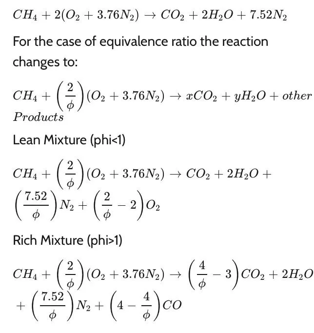
Reactions taking place at the constant pressure to calculate the coefficients

The relaxation factor we have taken is 0.2 for this case becuase it is under relaxation and value dont over shoot till the 0.9 value and when we further increases the value of relaxation factor 1. when we further increases the value after 1 the value overshoots and diverges the solution.
Program on Python to calculate the AFT of methane at different equivalence ratio:
"""
In this program we are calculating AFT of methane at different equivalence ratios
CH4 + 2(O2 + 3.76N2) = CO2 + 2H2O + 7.52N2
"""
import math
import matplotlib.pyplot as plt
import numpy as np

def h(T,co_effs):
	"""
	Function to evaulate enthalpy
	"""
	R = 8.314 #J/mol-K
	a1 = co_effs[0]
	a2 = co_effs[1]
	a3 = co_effs[2]
	a4 = co_effs[3]
	a5 = co_effs[4]
	a6 = co_effs[5]

	return (a1 + a2*T/2 + a3*pow(T,2)/3 + a4*pow(T,3)/4 + a5*pow(T,4)/5 + a6/T)*R*T

CH4_co_effs_l = [5.14987613E+00, -1.36709788E-02, 4.91800599E-05, -4.84743026E-08, 1.66693956E-11, -1.02466476E+04, -4.64130376E+00]
O2_co_effs_l = [3.78245636E+00, -2.99673416E-03, 9.84730201E-06, -9.68129509E-09, 3.24372837E-12, -1.06394356E+03, 3.65767573E+00]
N2_co_effs_h = [0.02926640E+02, 0.14879768E-02, -0.05684760E-05, 0.10097038E-09, -0.06753351E-13, -0.09227977E+04, 0.05980528E+02]
N2_co_effs_l = [0.03298677E+02, 0.14082404E-02, -0.03963222E-04, 0.05641515E-07, -0.02444854E-10, -0.10208999E+04, 0.03950372E+02]
CO2_co_effs_h = [3.85746029E+0, 4.41437026E-03, -2.21481404E-06, 5.23490188E-10, -4.72084164E-14, -4.87591660E+04, 2.27163806E+00]
H2O_co_effs_h = [3.03399249E+00, 2.17691804E-03, -1.64072518E-07, -9.70419870E-11, 1.68200992E-14, -3.00042971E+04, 4.96677010E+00]
O2_co_effs_h = [ 3.28253784E+00, 1.48308754E-03, -7.57966669E-07, 2.09470555E-10, -2.16717794E-14, -1.08845772E+03, 5.45323129E+00]
CO_co_effs_h = [2.71518561E+00, 2.06252743E-03, -9.98825771E-07, 2.30053008E-10, -2.03647716E-14, -1.41518724E+04, 7.81868772E+00]


def f(T,phi):
	R = 8.314 #J/mol-K
	"""
	Function that represents the Root finding problem
	"""
	if(phi<=1):
		h_CO2_p = h(T,CO2_co_effs_h)
		h_N2_p = h(T,N2_co_effs_h)
		h_H2O_p = h(T,H2O_co_effs_h)
		h_O2_p = h(T,O2_co_effs_h)

		H_products = h_CO2_p + 2*h_H2O_p + (7.52/phi)*h_N2_p + (2*phi-2)*h_O2_p
		n_products = 1 + 2 + 3.76*(2/phi) + (2/phi-2)

	else:
		h_CO2_p = h(T,CO2_co_effs_h)
		h_N2_p = h(T,N2_co_effs_h)
		h_H2O_p = h(T,H2O_co_effs_h)
		h_CO_p = h(T,CO_co_effs_h)

		H_products = (4/phi-3)*h_CO2_p + 2*h_H2O_p + (7.52/phi)*h_N2_p + (4-4/phi)*h_CO_p
		n_products = (4/phi-3) + 2 + (4-4/phi) + (7.52/phi)


	print(H_products)

	Tstd = 298.15
	h_CH4_r = h(Tstd,CH4_co_effs_l)
	h_O2_r = h(Tstd,O2_co_effs_l)
	h_N2_r = h(Tstd,N2_co_effs_l)

	H_rectants = h_CH4_r + (2/phi)*h_O2_r + (7.52/phi)*h_N2_r
	n_rectants = 1 + (2/phi) + 3.76*(2/phi)
	print(H_rectants)

	return (H_products - H_rectants) - R*(n_products*T-n_rectants*Tstd)

def fprime(T,phi):
	return (f(T+1e-6,phi) - f(T,phi))/1e-6

T_guess = 1500

tol = 1e-3
ct = 0
alpha = 0.2

phi = np.linspace(0.1,1.5,20)
T = []

for i in range (0,len(phi)):

	while(abs(f(T_guess,phi[i])) > tol):
		T_guess = T_guess - alpha*((f(T_guess,phi[i])/fprime(T_guess,phi[i])))
	T.append(T_guess)
plt.plot(phi,T,'*',color ='red')
print(T_guess,phi)
ct = ct+1

print(ct)
print(T_guess,phi)
plt.xlabel('Equivalence ratio')
plt.ylabel('Adiabatic flame Temperature')
plt.title('Effect of Euivalence ratio on AFT')
plt.grid('on')
plt.show()
Output got from the above code:
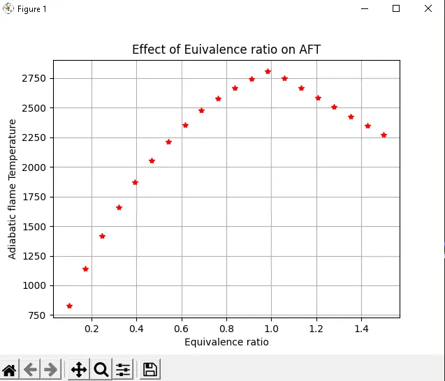
We run the code after and we got this graph sucessfully, This graph clearly shows that the Temperature get increases with increase in equivalence ratio till 1 and after that it decreases. So, we can conclude that from this study that at the Stiochiomtery mixture we got the maximum value of AFT i.e, Adiabatic Flame temperature and it gets low when we increase the fuel or air quantity or we can say that for the Lean or rich mixture we get the low AFT value. For this study we get maximum AFT value of stiohiometry mixture 2850K
Program on Cantera:
Cantera is an open-source collection of object-oriented software tools for problems involving chemical kinetics, thermodynamics, and transport processes. Among other things, it can be used to:
- Evaluate thermodynamic and transport properties of mixtures
- Compute chemical equilibrium
- Evaluate species chemical production rates
- Conduct kinetics simulations with large reaction mechanisms
- Simulate one-dimensional flames
- Conduct reaction path analysis
- Create process simulations using networks of stirred reactors
- Model non-ideal fluids
In cantera gas.TPX is an inbuilt function in Cantera and used in intialize the temperature, pressure and mole fraction for the each species. gas.set_equivalence_ratio is used to the give the equivalence ratio for the each spcies and gas in the used in Chemical kinetics.
Code for same problem in Cantera:
import matplotlib.pyplot as plt
import cantera as ct

"""
In this program we are calculating AFT of methane at different equivalence ratios
CH4 + 2(O2 + 3.76N2) = CO2 + 2H2O + 7.52N2
"""
gas = ct.Solution('gri30.xml')
phi = 0.1
for i in range (0,15):
	gas.TPX = 298.15,101325,{'CH4':1,'O2':2/phi,'N2':7.52/phi}
	gas.set_equivalence_ratio(phi,'CH4','O2:1,N2:3.76')
	gas.equilibrate('UV','auto')
	print(phi,gas.T)
	plt.plot(phi,gas.T,'*',color = 'blue')
	phi = phi+0.1

plt.xlabel('Equivalence Ratio')
plt.ylabel('Adiabatic Flame Temperature')
plt.title('Effect of Equivalence ratio on AFT using Cantera')
plt.grid('on')
plt.show()
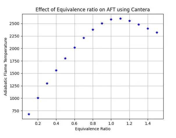
From this graph we can conclude that the maximum Flame temperature we got is 2600K that is low as compared to the Flame temperature we got from the python program that is may be due to Cantera solves on the Gibbs free energy for the combustion to reach the equilibruim state. Cantera contains Chemical library which consists GRI mechanism and also it contains thermodynamic properties already for chemical kinetics.
Case2:Flame temperature variation with Heat loss (In constant pressure-chamber)
Heat loss is considered as a constant pressure reactor with heat loss. The reactor is initially set at STP conditions that's why reaction is not going to take place to be an adiabatic reaction.
The stiochiometry reaction for methane-air combustion can be written as:

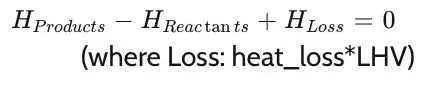
The heat loss in the program can be calculated from the lower heating value LHV. LHV can be obtained as the difference of products and reactants:

The heat loss factor is varied no heat loss to entire heat loss as a multiplier of LHV. the heat loss and enthalpy eqn is:
Program on python to calculate the AFT of methane with heat loss:
"""
In this program we are calculating AFT of methane at different equivalence ratios with heat loss
CH4 + 2(O2 + 3.76N2) = CO2 + 2H2O + 7.52N2
"""
import math
import matplotlib.pyplot as plt
import numpy as np

def h(T,co_effs):
	"""
	Function to evaulate enthalpy
	"""
	R = 8.314 #J/mol-K
	a1 = co_effs[0]
	a2 = co_effs[1]
	a3 = co_effs[2]
	a4 = co_effs[3]
	a5 = co_effs[4]
	a6 = co_effs[5]

	return (a1 + a2*T/2 + a3*pow(T,2)/3 + a4*pow(T,3)/4 + a5*pow(T,4)/5 + a6/T)*R*T

CH4_co_effs_l = [5.14987613E+00, -1.36709788E-02, 4.91800599E-05, -4.84743026E-08, 1.66693956E-11, -1.02466476E+04, -4.64130376E+00]
O2_co_effs_l = [3.78245636E+00, -2.99673416E-03, 9.84730201E-06, -9.68129509E-09, 3.24372837E-12, -1.06394356E+03, 3.65767573E+00]
N2_co_effs_h = [0.02926640E+02, 0.14879768E-02, -0.05684760E-05, 0.10097038E-09, -0.06753351E-13, -0.09227977E+04, 0.05980528E+02]
N2_co_effs_l = [0.03298677E+02, 0.14082404E-02, -0.03963222E-04, 0.05641515E-07, -0.02444854E-10, -0.10208999E+04, 0.03950372E+02]
CO2_co_effs_h = [3.85746029E+0, 4.41437026E-03, -2.21481404E-06, 5.23490188E-10, -4.72084164E-14, -4.87591660E+04, 2.27163806E+00]
H2O_co_effs_h = [3.03399249E+00, 2.17691804E-03, -1.64072518E-07, -9.70419870E-11, 1.68200992E-14, -3.00042971E+04, 4.96677010E+00]
O2_co_effs_h = [ 3.28253784E+00, 1.48308754E-03, -7.57966669E-07, 2.09470555E-10, -2.16717794E-14, -1.08845772E+03, 5.45323129E+00]
CO_co_effs_h = [2.71518561E+00, 2.06252743E-03, -9.98825771E-07, 2.30053008E-10, -2.03647716E-14, -1.41518724E+04, 7.81868772E+00]

def f(T,h_loss):
	Tstd = 298.15
	LHV = 800950

	h_CO2_p = h(T,CO2_co_effs_h)
	h_N2_p = h(T,N2_co_effs_h)
	h_H2O_p = h(T,H2O_co_effs_h)

	H_products = h_CO2_p + 2*h_H2O_p + (7.52)*h_N2_p

	print(H_products)

	h_CH4_r = h(Tstd,CH4_co_effs_l)
	h_O2_r = h(Tstd,O2_co_effs_l)
	h_N2_r = h(Tstd,N2_co_effs_l)

	H_rectants = h_CH4_r + (2)*h_O2_r + (7.52)*h_N2_r

	print(H_rectants)
	loss = h_loss*LHV
	return H_products - H_rectants + loss

def fprime(T,h_loss):
	return (f(T+1e-6,h_loss) - f(T,h_loss))/1e-6

T_guess = 1500

tol = 1e-3
ct = 0
alpha = 0.2

h_loss = np.linspace(0,1,20)
T_aft = [] #required temperature

for i in range (0,len(h_loss)):

		while(abs(f(T_guess,h_loss[i])) > tol):
			T_guess = T_guess - alpha*(f(T_guess,h_loss[i])/fprime(T_guess,h_loss[i]))
			ct = ct+1
		T_aft.append(T_guess)

plt.plot(h_loss,T_aft,'*',color ='red')

print(T_aft)
print(ct)
print(T_guess,h_loss)
plt.xlabel('Heat loss factor')
plt.ylabel('Flame Temperature (K)')
plt.title('Effect of Heat Loss on Flame Temperature')
plt.grid('on')
plt.show()
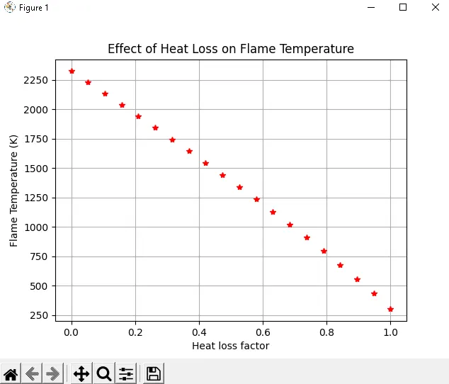
From this graph we can conclude that the as the heat is removed from the system the Adiabatic flame temperature of the combustion is reduced which is shows that the solution we got from this study is relevent and correct. The maximum temperature we got 2350K at 0 heat loss and at the maximum heat loss i.e, 1 for thsi case we got minimum temperature 298K.
Case3:Adiabatic flame temperature variation with respect to Alkane, Alkene, Alkyne:
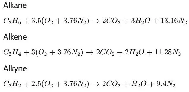
In this case we consider Alkane, Alkene and Alkynes for the reaction wi the heat loss 35% and here, are the reactions:
Program on Python to calculate the AFT w.r.t the Alkane, Alkene and Alkynes.
"""
In this program we are calculating AFT variation with respect to Alkane, Alkene and alkyne with 2 Carbon atoms
"""
import math
import matplotlib.pyplot as plt
import numpy as np

def h(T,co_effs):
	"""
	Function to evaulate enthalpy
	"""
	R = 8.314 #J/mol-K

	a1 = co_effs[0]
	a2 = co_effs[1]
	a3 = co_effs[2]
	a4 = co_effs[3]
	a5 = co_effs[4]
	a6 = co_effs[5]

	return (a1 + a2*T/2 + a3*pow(T,2)/3 + a4*pow(T,3)/4 + a5*pow(T,4)/5 + a6/T)*R*T

O2_co_effs_l = [3.78245636E+00, -2.99673416E-03, 9.84730201E-06, -9.68129509E-09, 3.24372837E-12, -1.06394356E+03, 3.65767573E+00]
N2_co_effs_h = [0.02926640E+02, 0.14879768E-02, -0.05684760E-05, 0.10097038E-09, -0.06753351E-13, -0.09227977E+04, 0.05980528E+02]
N2_co_effs_l = [0.03298677E+02, 0.14082404E-02, -0.03963222E-04, 0.05641515E-07, -0.02444854E-10, -0.10208999E+04, 0.03950372E+02]
CO2_co_effs_h = [3.85746029E+0, 4.41437026E-03, -2.21481404E-06, 5.23490188E-10, -4.72084164E-14, -4.87591660E+04, 2.27163806E+00]
H2O_co_effs_h = [3.03399249E+00, 2.17691804E-03, -1.64072518E-07, -9.70419870E-11, 1.68200992E-14, -3.00042971E+04, 4.96677010E+00]
O2_co_effs_h = [ 3.28253784E+00, 1.48308754E-03, -7.57966669E-07, 2.09470555E-10, -2.16717794E-14, -1.08845772E+03, 5.45323129E+00]
CO_co_effs_h = [2.71518561E+00, 2.06252743E-03, -9.98825771E-07, 2.30053008E-10, -2.03647716E-14, -1.41518724E+04, 7.81868772E+00]
C2H6_co_effs_l = [4.29142492E+00, -5.50154270E-03, 5.99438288E-05, -7.08466285E-08, 2.68685771E-11, -1.15222055E+04, 2.66682316E+00]
C2H4_co_effs_l = [3.95920148E+00, -7.57052247E-03, 5.70990292E-05, -6.91588753E-08, 2.69884373E-11, 5.08977593E+03, 4.09733096E+00]
C2H2_co_effs_l = [8.08681094E-01, 2.33615629E-02,-3.55171815E-05, 2.80152437E-08, -8.50072974E-12, 2.64289807E+04, 1.39397051E+01]

"""
Alkane
"""

def f_Alkane(T):
	R = 8.314 #J/mol-K
	Tstd = 298.15
	LHV = 1428275
	"""
	Function that represents the Root finding problem
	"""

	h_CO2_p = h(T,CO2_co_effs_h)
	h_N2_p = h(T,N2_co_effs_h)
	h_H2O_p = h(T,H2O_co_effs_h)

	h_C2H6_r =  h(Tstd,C2H6_co_effs_l)
	h_O2_r = h(Tstd,O2_co_effs_l)
	h_N2_r = h(Tstd,N2_co_effs_l)

	H_products = 2*h_CO2_p + 3*h_H2O_p + 13.16*h_N2_p
	H_rectants = h_C2H6_r + 3.5*h_O2_r + 13.16*h_N2_r

	return (H_products - H_rectants) + (0.35*LHV)

def fprime_Alkane(T):
	return (f_Alkane(T+1e-6) - f_Alkane(T))/1e-6
"""
Alkene
"""

def f_Alkene(T):
	R = 8.314 #J/mol-K
	Tstd = 298.15
	LHV = 1428275
	"""
	Function that represents the Root finding problem
	"""

	h_CO2_p = h(T,CO2_co_effs_h)
	h_N2_p = h(T,N2_co_effs_h)
	h_H2O_p = h(T,H2O_co_effs_h)

	h_C2H4_r =  h(Tstd,C2H4_co_effs_l)
	h_O2_r = h(Tstd,O2_co_effs_l)
	h_N2_r = h(Tstd,N2_co_effs_l)

	H_products = 2*h_CO2_p + 2*h_H2O_p + 11.28*h_N2_p
	H_rectants = h_C2H4_r + 3*h_O2_r + 11.28*h_N2_r

	return (H_products - H_rectants) + (0.35*LHV)

def fprime_Alkene(T):
	return (f_Alkene(T+1e-6) - f_Alkene(T))/1e-6

"""
Alkyne
"""

def f_Alkyne(T):
	R = 8.314 #J/mol-K
	Tstd = 298.15
	LHV = 1428275
	"""
	Function that represents the Root finding problem
	"""

	h_CO2_p = h(T,CO2_co_effs_h)
	h_N2_p = h(T,N2_co_effs_h)
	h_H2O_p = h(T,H2O_co_effs_h)

	h_C2H2_r =  h(Tstd,C2H2_co_effs_l)
	h_O2_r = h(Tstd,O2_co_effs_l)
	h_N2_r = h(Tstd,N2_co_effs_l)

	H_products = 2*h_CO2_p + h_H2O_p + 9.4*h_N2_p
	H_rectants = h_C2H2_r + 2.5*h_O2_r + 11.28*h_N2_r

	return (H_products - H_rectants) + (0.35*LHV)

def fprime_Alkyne(T):
	return (f_Alkyne(T+1e-6) - f_Alkyne(T))/1e-6

T_Alkane_guess = 1500
T_Alkene_guess = 1500
T_Alkyne_guess = 1500

tol = 1e-3
#ct = 0
alpha = 0.2

#phi = np.linspace(0.1,1.5,20)
T = []

#for i in range (0,len(phi)):

"""
Alkane
"""
while(abs(f_Alkane(T_Alkane_guess)) > tol):
	T_Alkane_guess = T_Alkane_guess - alpha*(f_Alkane(T_Alkane_guess)/fprime_Alkane(T_Alkane_guess))
T.append(T_Alkane_guess)

"""
Alkene
"""
while(abs(f_Alkene(T_Alkene_guess)) > tol):
	T_Alkene_guess = T_Alkene_guess - alpha*(f_Alkene(T_Alkene_guess)/fprime_Alkene(T_Alkene_guess))
T.append(T_Alkene_guess)

"""
Alkyne
"""
while(abs(f_Alkyne(T_Alkyne_guess)) > tol):
	T_Alkyne_guess = T_Alkyne_guess - alpha*(f_Alkyne(T_Alkyne_guess)/fprime_Alkyne(T_Alkyne_guess))
T.append(T_Alkyne_guess)

Fuel = ['Alkane', 'Alkene', 'Alkyne']

print(T)
plt.bar(Fuel,T,color = 'red', width = 0.4)
plt.xlabel('Type of Hydrocarbon')
plt.ylabel('Adiabatic flame Temperature')
plt.title('AFT variation w.r.t Hydrocarbons')
plt.show() 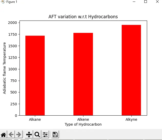
From this graph we can conclude that the minimum AFT is for Alkane and the Maximum AFT is for Alkyne. This is may be due to the Triple carbon carbon bonding in the Alkynes that is why to break the bond or to take place the reaction temperature is required is more as compared for the Alkane's. The flame temperature for the ethane is 1650K, for ethene is 1785K and for the ethyne is around 1900K
Case4: Adiabatic flame temperature variation with respect to number of Carbon atom chains :
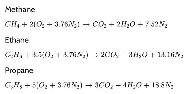
In this case we increased the carbon atoms in alkane's and then study the variation in the AFT here are the reactions:
Program on pyhton to calculate the AFT variation w.r.t number of carbon atoms:
"""
In this program we are calculating AFT variation with respect to number of Carbon Atoms
"""
import math
import matplotlib.pyplot as plt
import numpy as np

def h(T,co_effs):
	"""
	Function to evaulate enthalpy
	"""
	R = 8.314 #J/mol-K

	a1 = co_effs[0]
	a2 = co_effs[1]
	a3 = co_effs[2]
	a4 = co_effs[3]
	a5 = co_effs[4]
	a6 = co_effs[5]

	return (a1 + a2*T/2 + a3*pow(T,2)/3 + a4*pow(T,3)/4 + a5*pow(T,4)/5 + a6/T)*R*T

CH4_co_effs_l = [5.14987613E+00, -1.36709788E-02, 4.91800599E-05, -4.84743026E-08, 1.66693956E-11, -1.02466476E+04, -4.64130376E+00]
O2_co_effs_l = [3.78245636E+00, -2.99673416E-03, 9.84730201E-06, -9.68129509E-09, 3.24372837E-12, -1.06394356E+03, 3.65767573E+00]
N2_co_effs_h = [0.02926640E+02, 0.14879768E-02, -0.05684760E-05, 0.10097038E-09, -0.06753351E-13, -0.09227977E+04, 0.05980528E+02]
N2_co_effs_l = [0.03298677E+02, 0.14082404E-02, -0.03963222E-04, 0.05641515E-07, -0.02444854E-10, -0.10208999E+04, 0.03950372E+02]
CO2_co_effs_h = [3.85746029E+0, 4.41437026E-03, -2.21481404E-06, 5.23490188E-10, -4.72084164E-14, -4.87591660E+04, 2.27163806E+00]
H2O_co_effs_h = [3.03399249E+00, 2.17691804E-03, -1.64072518E-07, -9.70419870E-11, 1.68200992E-14, -3.00042971E+04, 4.96677010E+00]
O2_co_effs_h = [ 3.28253784E+00, 1.48308754E-03, -7.57966669E-07, 2.09470555E-10, -2.16717794E-14, -1.08845772E+03, 5.45323129E+00]
CO_co_effs_h = [2.71518561E+00, 2.06252743E-03, -9.98825771E-07, 2.30053008E-10, -2.03647716E-14, -1.41518724E+04, 7.81868772E+00]
C2H6_co_effs_l = [4.29142492E+00, -5.50154270E-03, 5.99438288E-05, -7.08466285E-08, 2.68685771E-11, -1.15222055E+04, 2.66682316E+00]
C3H8_co_effs_l = [0.93355381E+00, 0.26424579E-01, 0.61059727E-05, -0.21977499E-07, 0.95149253E-11, -0.13958520E+05, 0.19201691E+02]

"""
Methane
"""

def f_Methane(T):
	R = 8.314 #J/mol-K
	Tstd = 298.15

	"""
	Function that represents the Root finding problem
	"""

	h_CO2_p = h(T,CO2_co_effs_h)
	h_N2_p = h(T,N2_co_effs_h)
	h_H2O_p = h(T,H2O_co_effs_h)

	h_CH4_r =  h(Tstd,CH4_co_effs_l)
	h_O2_r = h(Tstd,O2_co_effs_l)
	h_N2_r = h(Tstd,N2_co_effs_l)

	H_products = h_CO2_p + 2*h_H2O_p + 7.52*h_N2_p
	H_rectants = h_CH4_r + 2*h_O2_r + 7.52*h_N2_r

	return (H_products - H_rectants)

def fprime_Methane(T):
	return (f_Methane(T+1e-6) - f_Methane(T))/1e-6


"""
Ethane
"""

def f_Ethane(T):
	R = 8.314 #J/mol-K
	Tstd = 298.15

	"""
	Function that represents the Root finding problem
	"""

	h_CO2_p = h(T,CO2_co_effs_h)
	h_N2_p = h(T,N2_co_effs_h)
	h_H2O_p = h(T,H2O_co_effs_h)

	h_C2H6_r =  h(Tstd,C2H6_co_effs_l)
	h_O2_r = h(Tstd,O2_co_effs_l)
	h_N2_r = h(Tstd,N2_co_effs_l)

	H_products = 2*h_CO2_p + 3*h_H2O_p + 13.16*h_N2_p
	H_rectants = h_C2H6_r + 3.5*h_O2_r + 13.16*h_N2_r

	return (H_products - H_rectants)

def fprime_Ethane(T):
	return (f_Ethane(T+1e-6) - f_Ethane(T))/1e-6


"""
Propane
"""

def f_Propane(T):
	R = 8.314 #J/mol-K
	Tstd = 298.15

	"""
	Function that represents the Root finding problem
	"""

	h_CO2_p = h(T,CO2_co_effs_h)
	h_N2_p = h(T,N2_co_effs_h)
	h_H2O_p = h(T,H2O_co_effs_h)

	h_C3H8_r =  h(Tstd,C3H8_co_effs_l)
	h_O2_r = h(Tstd,O2_co_effs_l)
	h_N2_r = h(Tstd,N2_co_effs_l)

	H_products = 3*h_CO2_p + 4*h_H2O_p + 18.8*h_N2_p
	H_rectants = h_C3H8_r + 5*h_O2_r + 18.8*h_N2_r

	return (H_products - H_rectants)

def fprime_Propane(T):
	return (f_Propane(T+1e-6) - f_Propane(T))/1e-6

T_Methane_guess = 1500
T_Ethane_guess = 1500
T_Propane_guess = 1500

tol = 1e-3
#ct = 0
alpha = 0.2

#phi = np.linspace(0.1,1.5,20)
T = []

#for i in range (0,len(phi)):

"""
Methane
"""

while(abs(f_Methane(T_Methane_guess)) > tol):
	T_Methane_guess = T_Methane_guess - alpha*(f_Methane(T_Methane_guess)/fprime_Methane(T_Methane_guess))
T.append(T_Methane_guess)

"""
Ethane
"""
while(abs(f_Ethane(T_Ethane_guess)) > tol):
	T_Ethane_guess = T_Ethane_guess - alpha*(f_Ethane(T_Ethane_guess)/fprime_Ethane(T_Ethane_guess))
T.append(T_Ethane_guess)

"""
Propane
"""
while(abs(f_Propane(T_Propane_guess)) > tol):
	T_Propane_guess = T_Propane_guess - alpha*(f_Propane(T_Propane_guess)/fprime_Propane(T_Propane_guess))
T.append(T_Propane_guess)

Fuel = ['Methane', 'Ethane', 'Propane']

print(T)
plt.bar(Fuel,T,color = 'red', width = 0.4)
plt.xlabel('Number of Carbon Atoms')
plt.ylabel('Adiabatic flame Temperature')
plt.title('AFT variation w.r.t number of Carbon atoms')
plt.show()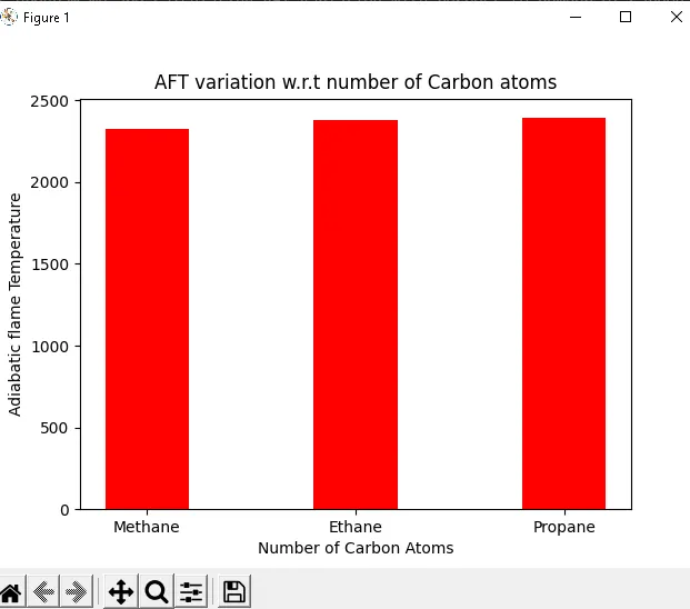
From this graph we can clearly, see that the as the number of carbon atoms increases the temperature is going to increase that is due to the energy required to break the carbon atoms bonds in the reaction. The flame temperature for Methane is 2325.9K, for Ethane is 2379.8K and for Propane is 2392.9K.
Conclusion:-
- From this study we can conclude that the Maximum Adiabatic Flame Temperature we got for the stiochiometry mixture as compared For the Lean and rich mixture's.
- If there is heat is loss the temperature gets reduced that is because the heat is loss from the system or removed from the sytem.
- The AFT is more for the Alkynes as compared to the Alkane's and Alkene's that is due to the triple bonding of C-C atoms the energy is required more for reaction taking place.
- In the last case increase in the carbon atoms we got the high flame temperature for propane that is due to an increase in hydrogen and Carbon atoms.
- For the First case we have used two approaches Python and Cantera: In the python case we got the maximum Adiabatic Flame temperature at 2850K and In the Cantera we got the maximum AFT at 2600K It shows difference this is because Cantera solves by reducing the Gibbs free energy of the equation.