Week 3.5 - Deriving 4th order approximation of a 2nd order derivative using Taylor Table method

AIM: Write a program in Matlab to evaluate the second-order derivative of the analytical function exp(x)*cos(x) and compare it with the 3 numerical approximations that we have derived.

OBJECTIVE: Derive the following 4th order approximations of the second-order derivative.

• Central difference
• Skewed right-sided difference
• Skewed left-sided difference

THEORY:

The fourth order approximations and derivative of second order and the calculations is done in the below:

Central difference is an average of the forward and backward differences. ... If the data values are available both in the past and in the future, the numerical derivative should be approximated by the central difference.Using this, one can find an approximation for the derivative of a function at a given two points.

Right skewed:It takes the points from the refrence points only in the right hand side and It is also known as forward difference.

Left skewed:It takes the points from the refrence points only in the left hand side and It is also known as backward difference.

Here the calculation for the cental difference scheme by taylor table method to find out the unknown coefficients:

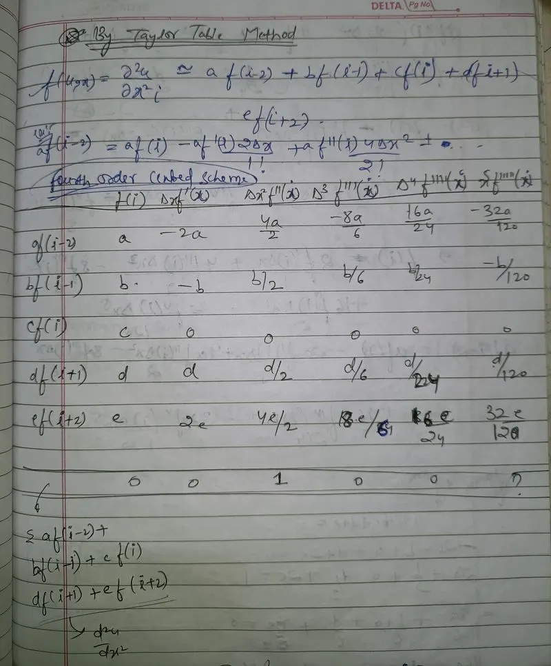
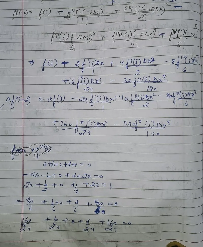
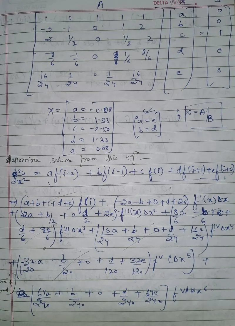
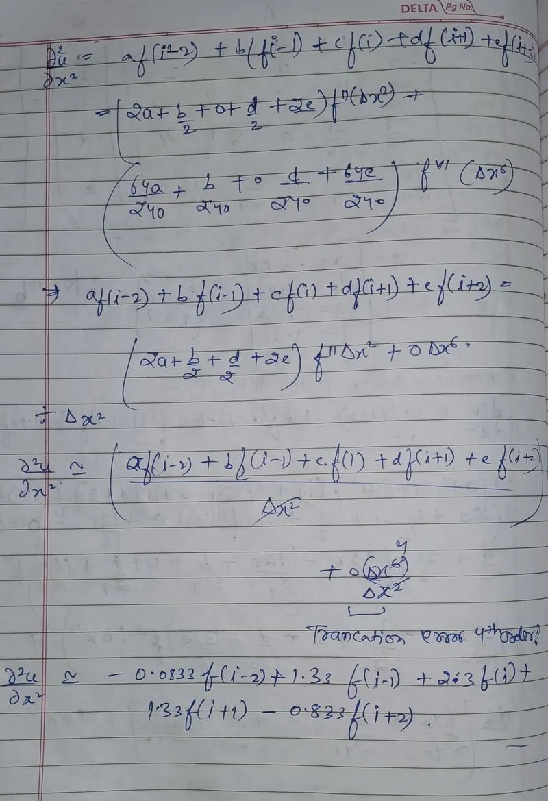
Similarly, we have to calculate for the right skewed and left skewed scheme by taylor table method to find out the cofficients:

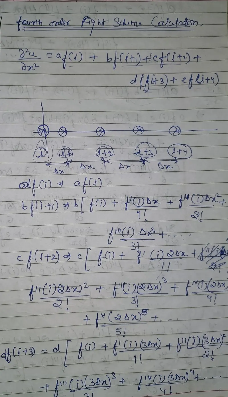
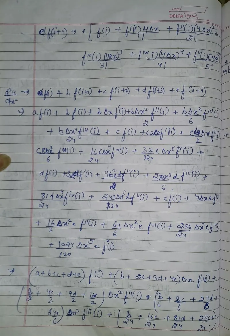
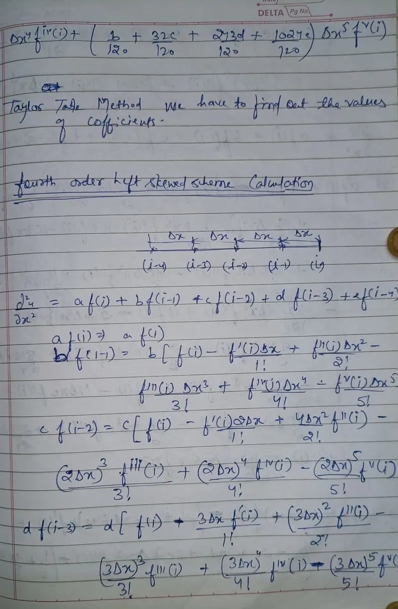
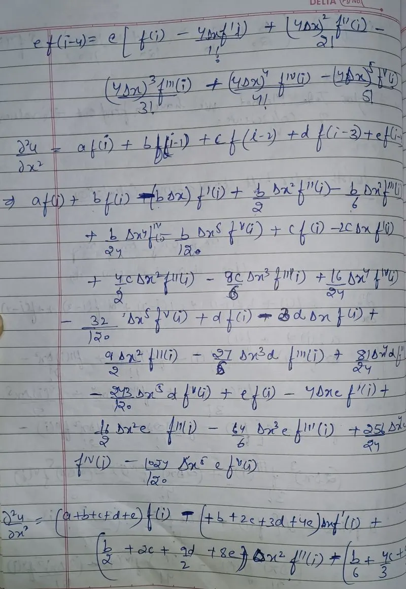
here is the taylor table for left skewed and right skewed and similar as the central difference, hence rest of the calculation has done by code :

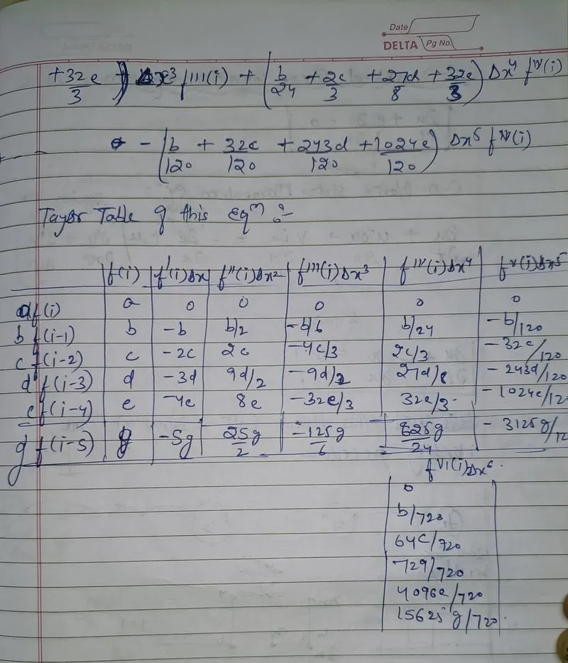
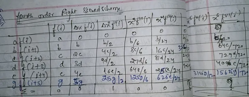
In the taylor table the column of del sqaure of x *f"(i) its summation is equal to 1 it is just because we have to obtain the second order derivative of this function.

Reason behind the take no. of coefficients difference in central difference than the right skewed and Left skewed:

In central differencing, we have to keep no. of points for the stencil is in symmteric form. It is just because the left hand side of refrence point and right hand side the of refrence point number of points must be equal.and If it is not done the stencil becomes unsymmetric and hence we have to take no. of data points is in odd form.

Here is the main Octave code where is the matrixes has been solved and find out the coefficients and after find out the coefficients error we have to find between the analytical derivative and numerical derivate and plots the error graph.

clear all
close all
clc

x = pi/3;
dx = linspace(pi/4,pi/400,20);

%f(x) = e^(x)*cos(x)
%f'(x) = -e^(x)*sin(x) + e^(x)*cos(x)
%f''(x) = -2*e^(x)*sin(x)

analytical_derivative = -2*e^(x)*sin(x);

f = @(x) e^x*cos(x) %Function handle 

for i=1:length(dx)
  
right_error(i) = right_skewed(x,dx(i),analytical_derivative,f);
left_error(i) = left_skewed(x,dx(i),analytical_derivative,f);
central_error(i) = central(x,dx(i),analytical_derivative,f);

end
figure(1)
loglog(dx,right_error)
hold on
loglog(dx,left_error,'r')
loglog(dx,central_error,'b')
legend('right_error','left_error','central_error')

Here is the right skewed, left skewed and central difference function codes that is paas in the main program and help for the finding out the unknown coefficients and finot out the error between the anaytical derivative and numerical derivate.

function error = right_skewed(x,dx,analytical_derivative,f)
  
% Right skewed scheme
A = [1 1 1 1 1 1; 0 1 2 3 4 5; 0 1/2 2 9/2 8 25/2; 0 1/6 4/3 27/6 64/6 125/6; 0 1/24 16/24 81/24 256/24 625/24; 0 1/120 32/120 243/120 1024/120 3125/120];
B = [0;0;1;0;0;0];

% AX=B
X = inv(A)*(B);

%Numerical derivative
%f"(x) = af(x) + bf(x+dx) + cf(x+2*(dx)) + df(x+3*(dx)) + ef(x+4*(dx) + gf(x+5*(dx)) 

Numerical_derivative = (X(1)*f(x) + X(2)*f(x+dx) + X(3)*f(x+2*dx) + X(4)*f(x+3*dx) + X(5)*f(x+4*dx) + X(6)*f(x+5*dx))/dx^2;
  
 
error = abs(analytical_derivative - Numerical_derivative);
  
  
  end

function error = left_skewed(x,dx,analytical_derivative,f)
  
% Left skewed scheme
A = [1 1 1 1 1 1 ; 0 -1 -2 -3 -4 -5; 0 1/2 2 9/2 8 25/2; 0 -1/6 -4/3 -9/2 -32/3 -125/6;0 1/24 2/3 27/8 32/3 625/24; 0 -1/120 -32/120 -243/120 -1024/120 -3125/120];
B = [0;0;1;0;0;0];

% AX=B
X = inv(A)*(B);

%Numerical derivative
%f"(x) = af(x) + bf(x-dx) + cf(x-2*(dx)) + df(x-3*(dx)) + ef(x-4*(dx)+gf(x-5*(dx)) 

Numerical_derivative = (X(1)*f(x) + X(2)*f(x-dx) + X(3)*f(x-2*dx) + X(4)*f(x-3*dx) + X(5)*f(x-4*dx) + X(6)*f(x-5*dx))/dx^2;
  
 
error = abs(analytical_derivative - Numerical_derivative);
  
  
  end

function error = central(x,dx,analytical_derivative,f)
  
%Central scheme
%A = [1 1 1 1 1; -2 -1 0 1 2; 2 1/2 0 1/2 2; -8/6 1/6 0 1/6 8/6; 16/24 1/24 0 1/24 16/24] Incorrect 4th and 5th row
A = [1,1,1,1,1;-2,-1,0,1,2;2,1/2,0,1/2,2;-8/6,-1/6,0,1/6,8/6;16/24,1/24,0,1/24,16/24];
B = [0;0;1;0;0];

% AX=B
X = inv(A)*(B);

%Numerical derivative
%f"(x) = af(x-2dx) + bf(x-dx) + cf(x) + df(x-dx) + ef(x-2dx) 
Numerical_derivative = (X(1)*f(x-2*dx) + X(2)*f(x-dx) + X(3)*f(x) + X(4)*f(x+dx) + X(5)*f(x+2*dx))/dx^2;
  
 
error = abs(analytical_derivative - Numerical_derivative);
  
end

The coeffcients we have placed in the equation plays a vital role in the approximation of the derivate and by the taylor table method it is easy to calculate the unknown coeffcients

Here is the plot we got from this code:

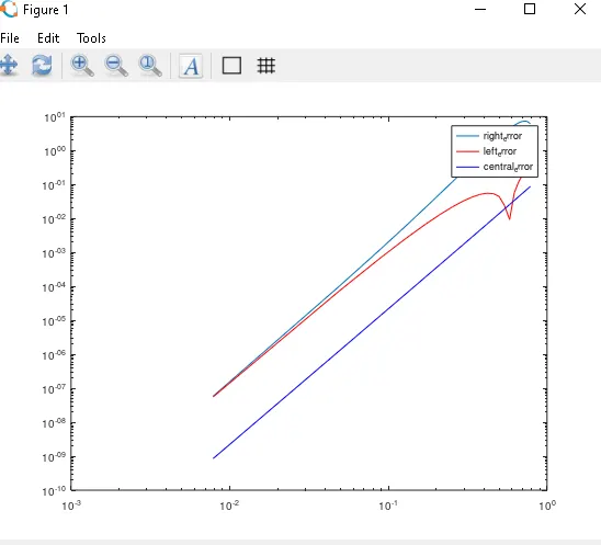
Conclusion from this graph : As the dx decreases the error is also decreases it follows this relationship dx is directly proptional to the error and as we seen In the plot the central differencing has very less error as compared to the right skewed and left skewed it is because it takes information from the both side of the nodes.

Why schemes are seem useful:when we have not any node at the boundry then skewed schemes are useful to approximate to improve the accuracy but we have interal nodes the central ones are good though.