Week 3 - Solving second order ODEs

AIM - To write a program on for simulating the transient behaviour of a simple pendulum.

OBJECTIVE:

To write a program that solves the following ODE. This ODE represents the equation of motion of a simple pendulum with damping.

THEORY:

ODE is used to describe the transient behaviour of a system. A simple example is a pendulum. the way pendulum moves its a newton 2nd law and when this law is written down , we get a 2nd order ODE to describe the postion of a bob w.r.t time.

This ODE represents the equation of motion of a simple pendulum.

L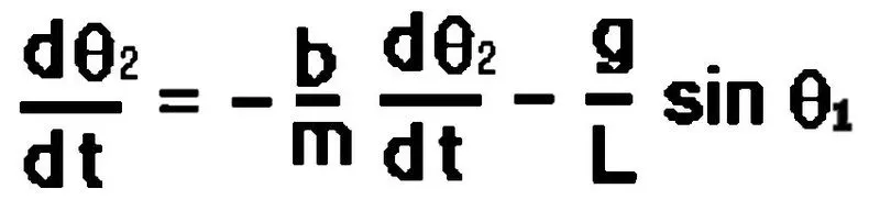

In the above equation,

g = gravity in m/s2,

L = length of the pendulum in m,

m = mass of the ball in kg,

b=damping coefficient.

given conditions are:-

L=1 metre,

m=1 kg,

b=0.05.

g=9.81 m/s2.

Simulate the motion between 0-20 sec, for angular displacement=0,angular velocity=3 rad/sec at time t=0.

program on MATLAB:

%write a program on for simulating the transient behaviour of simple pendulum.

clear all
close all
clc

%defining the input variables

b=0.05;
g=9.81;
l=1;
m=1;
ct=1;

%initial conditions
theta_0 = [0;3];
t_span = linspace(0,20,500)   %time

%solve ODE
[t,results] = ode45(@(t,theta) ode_func(t,theta,b,g,l,m),t_span,theta_0);

figure(1)
hold on
plot(t,results(:,1),'color','r')
plot(t,results(:,2),'color','b')
ylabel('position radians')
xlabel('angular velocity')

grid on

theta2 = results(:,1);

for i = 1:length(t);
    theta_x = results(i,1);   %theta_x keeps changing w.r.t time
    x0 = 0;
    y0 = 0; 
    
    x1 = l*sin(theta_x);
    y1 = -l*cos(theta_x);
    
    %plotting the pendulum
    figure(2)
    plot([-0.5,0.5 ],[0,0],'color','b','linewidth',5);
    hold on
    plot([x0 x1],[y0 y1],'color','r','linewidth',3);
    
    plot (x1,y1,'o','MarkerSize',15,'markerfacecolor','y')
    hold off
    grid on
   axis([-1.5 1.5 -1.5 0.5]);
    pause(0.002)
   M(ct) = getframe(gcf);
    ct = ct+1;
    
    
    
end
movie(M)
videofile = VideoWriter('ODE_1.avi','Uncompressed AVI');
open(videofile)
writeVideo(videofile,M)
close(videofile)

funtion code which is used in this program:

function [dtheta_dt] = ode_func(t,theta,b,g,l,m)

theta1 = theta(1)
theta2 = theta(2)
dtheta1_dt = theta2;
dtheta2_dt = -(b/m)*theta2 -(g/l)*sin(theta1);

dtheta_dt = [dtheta1_dt ; dtheta2_dt];

end

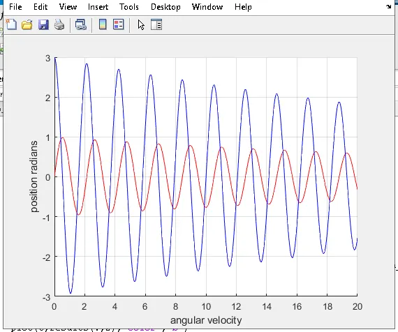
outputs we got from this program.

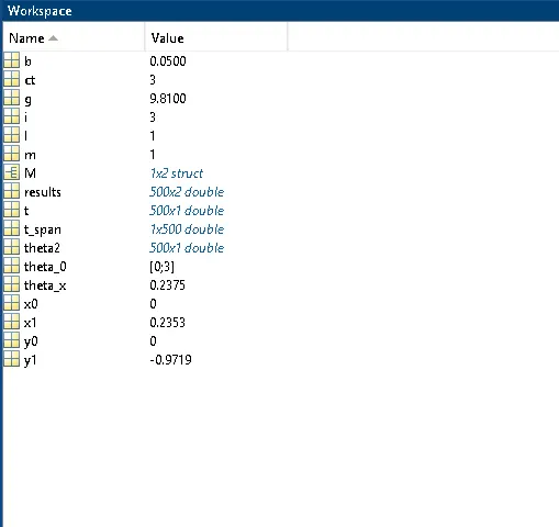
graph of displcement and velocity

STEPS

• first we have to break the higher order ODE into first order ODE.
• in main program the value of each is assigned. the ode45 is inbuild function or solver that is used to solve the ode for pendulum with damping.
• then we used the function for ODE of the pendulum to ease in solving of thr problem.

the ode45 solver in MATLAB solve the program and we got results that we are using to simulating the simple pendulum.

here is the link for the video:

https://youtu.be/s9Ti0SakMLI