Week 5.1 - Mid term project - Solving the steady and unsteady 2D heat conduction problem

AIM: Write a code to solve the 2D heat conduction equation by using the point iterative techniques for steady and transient state heat condcuction equation.

Objective: Implement the following methods for solving implicit equations.

• Jacobi
• Gauss-seidel
• Successive over-relaxation

Given inputs: Boundary conditions for the problem are as follows;

• Top Boundary = 600 K
• Bottom Boundary = 900 K
• Left Boundary = 400 K
• Right Boundary = 800 K
• Absolute error criteria is given 1e-4
• Length of domain = 1m

First we have to descritize the 2D steady state eqaution, so that it can be solved numerically. After descritizing this equation we have to solve the quation by 3 different iterative solvers example: jacobi method, Guass seidel and Successive over-relaxation method.

Here is the main concept we are going to solve by the help of iterative solver:

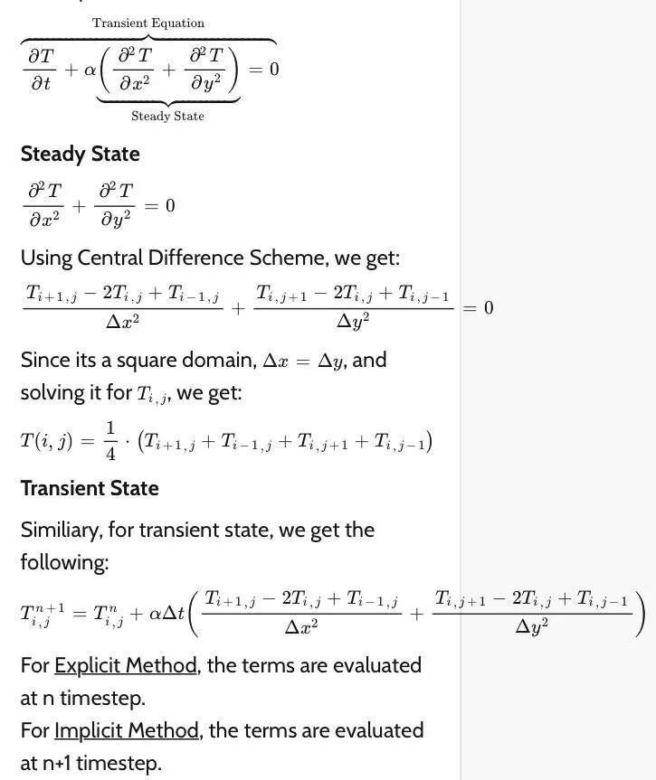
Here is the code to solve a steady state heat conduction equation:

%code to solve a 2D steady state heat conduction equation.
%(d^2T/dx^2)+(d^2T/dy^2) = 0
clear all
close all
clc

%inputs
l =1            %length of domain
nx = 10         %no. of grid points in x direction
ny = nx         %no. of grid points in y direction
w = 1.2         %omega (relaxation factor)
dx = l/(nx-1)   %grid size in the direction of x
dy = l/(ny-1)   %grid size in the direction of y


T = ones(nx,ny);    %temperature array
k = 2*((dx^2 + dy^2)/(dx^2*dy^2));   %defining the value of constant

%creating a copy of T
x = linspace(0,1,nx);
y = linspace(0,1,ny);

%boundary conditions given 
%top boundary temp (T_t)
T_t = 600
%bottom boundary temp (T_b)
T_b = 900
%left boundary temp (T_l)
T_l = 400
%right boundary temp (T_r)
T_r = 800

%updating the value of temp
T(:,1) = T_l;
T(:,nx) = T_r;
T(1,:) = T_t;
T(ny,:) = T_b;

Told = T;
Tinit=T;

%calculating the average temperatures
T(1,1) = (T_t + T_r)/2;
T(nx,ny) = (T_r + T_b)/2;
T(1,ny) = (T_t + T_r)/2;
T(nx,1) = (T_l + T_b)/2;

tol = 1e-4;   %tolerance value
error = 9e9;  %error value


%jacobi method

  jacobi_iter = 1;
while(error > tol)
      
      for i = 2:nx-1
           for j = 2:ny-1
         
             T(i,j) = 0.25*(Told(i-1,j) + Told(i+1,j) + Told(i,j-1)+Told(i,j+1)); 
             
          end         
     end
            
     error = max(max(abs(Told - T)));
     Told = T;
     jacobi_iter = jacobi_iter + 1;
     

end
figure(1)
contourf(x,fliplr(y),T);
colorbar;
xlabel('X axis')
ylabel('T')
title_text = sprintf('Steady State Jacobi Iteration number = %d',jacobi_iter);
title(title_text)
pause(0.03)

%Re-initializing the fields
T = Tinit;
Told = Tinit;
error=9e9;

%guass sedial method(GS)

  GS_iter = 1;
while(error > tol)
      
      for i = 2:nx-1
           for j = 2:ny-1
         
             T(i,j) = 0.25*(T(i-1,j) + Told(i+1,j) + T(i,j-1)+Told(i,j+1)); 
  
          end   
     end
   
            
     error = max(max(abs(Told -T)));
     Told = T;
     
     GS_iter = GS_iter + 1;
     

end
figure(2)
contourf(x,fliplr(y),T);
colorbar;
xlabel('X axis')
ylabel('T')
title_text = sprintf('Steady State GS Iteration number = %d',GS_iter);
title(title_text)

%Re-initializing the fields
T = Tinit;
Told = Tinit;
error=9e9;


%sucessive over relaxation(SOR)

  SOR_iter = 1;
while(error > tol)
      
      for i = 2:nx-1
           for j = 2:ny-1
         
            T(i,j) =   (1-w)*Told(i,j)  + (w*0.25*(T(i-1,j) + Told(i+1,j) + T(i,j-1)+Told(i,j+1))); 
   
         
         end
              
     end
   
            
     error = max(max(abs(Told -T)));
     Told = T;
   
  SOR_iter = SOR_iter + 1;
     

end
figure(3)
contourf(x,fliplr(y),T);
colorbar;
xlabel('X axis')
ylabel('T')
title_text = sprintf('Steady State SOR Iteration number = %d',SOR_iter);
title(title_text)

Report: 2D heat conduction equation for the steady state :

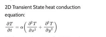
First we have to descritize the 2D steady state eqaution, so that it can be solved numerically. After descritizing this equation we have to solve the quation by 3 different iterative solvers example: jacobi method, Guass seidel and Successive over-relaxation method. and defining the inputs like L = 1m,omega = 1.2

Let consider a 2D domain where no. of grids points in x direction (nx) = 10 and no. of grids points in y direction (ny) is also 10 nx=ny. let the domain length is 1m and after this we have define the grid sizes of dx and dy.

After that we are going to generate a temperature array and generating an array of Temperature in x and y direction. Then we define the initial conditons as Tinitial = T and define the boundary conditions for the temperature as given in challenge.We are also calculate the corners temperatues by taking their averages. We are also giving the tolernce values that the space loop works below the given tolerance and calculating the error values between the Told-T.

Absolute error criteria is equal to 1e-4, the error in the solution is compared after each iterations with absolute error criteria and if it is more than the absolute error, then the iterations keep on going until the value of error is less than the absolute error criteria.

Jacobi method for steady state:

from the above formula we are going to calculate the Temperature at the each time steps in this method we know the old values of the Temperature like Top Boundary (T_t)= 600 K, Bottom Boundary (T_b)= 900 K, Left Boundary(T_l )= 400 K and Right Boundary(T_r) = 800 K. So for the first value of error we are going to calculate the Tn+1 by taking the told values.After first iteration the difference between Told and T has been calculated. If it is more than the absolute error criteria or tolerance value, then the iteration keeps on going until the difference is less than the tolerance. Told value is keep on updating after each iteration inside the convergence loop it is not updating while loop never exit.

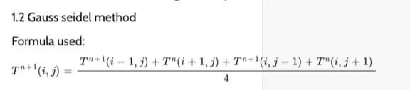
The above formula is also same as the jacobi method but there is one difference that when the first iteration is run to calculate the value for T at a node, then this updated value of T is going to use to calculate the value at the next node. and This method decreases the convergence time.

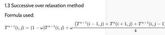
This formula is used for the both jacobi and GS methods,In this method we are going to introduce a new parameter called relaxation factor(omega). It is used which over estimates the value and leads to an increase value in T for each iteration, in this way the convergence is achieved much faster than the two methods.

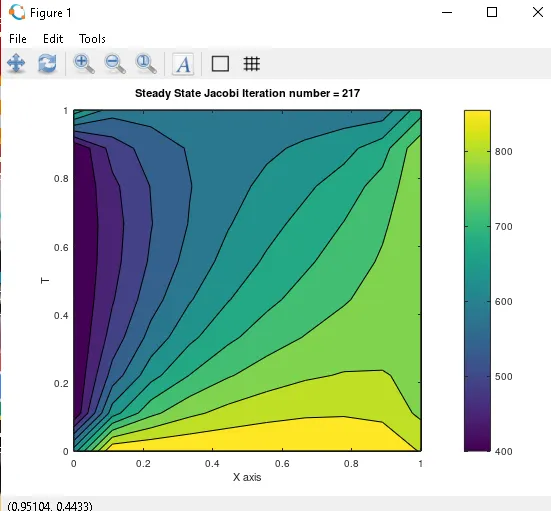
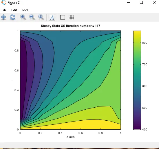
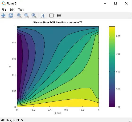
Plots for the above codes we got:

Conclusion:

• The above three plots shows the temperature distribution over a thin plate and also displays the number of iterations and analysis time.
• From the above plots we can say that jacobi method has a maximum number of iterations than the rest of the methods and convergence time is also more than the other methods.
• number of iterations and convergence time for Gauss seidel method is less than the jacobi method but more than SOR.
• The succesive over relaxation method has least number od iterations and it took least time for convergence.
• In steady state analysis SOR method is fastest.

Matlab/Octave code for solving 2D Transient state heat conduction equation by implicit method.

%code to solve a 2D steady state heat conduction equation
%dT/dt = alpha*((d^2T/dx^2) + (d^2T/dy^2)) 
clear all
close all
clc

%inputs
l =1      %length of domain
nx = 10   %no. of grid points in x direction
ny = nx  %no. of grid points in y direction
w = 1.2   %omega
dx = l/(nx-1)
dy = l/(ny-1)
alpha = 2;

T = ones(nx,ny);    %temperature array

%creating a copy of T
x = linspace(0,1,nx);
y = linspace(0,1,ny);

%boundary conditions given 
%top boundary temp (T_t)
T_t = 600
%bottom boundary temp (T_b)
T_b = 900
%left boundary temp (T_l)
T_l = 400
%right boundary temp (T_r)
T_r = 800

%updating the value of temp
T(:,1) = T_l;
T(:,nx) = T_r;
T(1,:) = T_t;
T(ny,:) = T_b;

Told = T;
Tprev = T;
Tinit = T;

%calculating the average temperatures
T(1,1) = (T_t + T_r)/2;
T(nx,ny) = (T_r + T_b)/2;
T(1,ny) = (T_t + T_r)/2;
T(nx,1) = (T_l + T_b)/2;

tol = 1e-4;   %tolerance value
error = 9e9;
conv = error;
dt = 1e-2;

k1 = alpha*dt/dx^2;
k2 = alpha*dt/dy^2;
cfl = k1+k2;
 jacobi_iter = 1;
 jacobi_time_iter=1;
%jacobi method

while(conv > tol)
error = 9e9;
while(error > tol)
      
      for i = 2:nx-1
           for j = 2:ny-1
         
             term1 = (1+2*k1+2*k2)^-1*Tprev(i,j);
             term2 =  (Told(i+1,j) + Told(i-1,j))*k1*(1+2*k1+2*k2)^-1;
             term3 = (Told(i,j+1) + Told(i,j-1))*k2*(1+2*k1+2*k2)^-1;
             T(i,j) = term1 + term2 + term3;
             
          end         
     end
            
     error = max(max(abs(Told - T)));
     Told = T;
     jacobi_iter = jacobi_iter + 1;
     
end
     conv = max(max(abs(Tprev - T)));
     Tprev = T;
     jacobi_time_iter = jacobi_time_iter + 1;

end
figure(1)
contourf(x,fliplr(y),T);
colorbar;
xlabel('X axis')
ylabel('T')
title_text = sprintf('Transient Implicit Jacobi Iteration number = %d',jacobi_iter);
title(title_text)


%Re-initializing the fields
T = Tinit;
Told = Tinit;
Tprev = Tinit;
error=9e9;
conv=error;

 gs_iter = 1;
 gs_time_iter=1;

while(conv > tol)
error = 9e9;
while(error > tol)
      
      for i = 2:nx-1
           for j = 2:ny-1
         
             term1 = (1+2*k1+2*k2)^-1*Tprev(i,j);
             term2 =  (Told(i+1,j) + T(i-1,j))*k1*(1+2*k1+2*k2)^-1;
             term3 = (Told(i,j+1) + T(i,j-1))*k2*(1+2*k1+2*k2)^-1;
             T(i,j) = term1 + term2 + term3;
             
          end         
     end
            
     error = max(max(abs(Told - T)));
     Told = T;
     gs_iter = gs_iter + 1;
     
end
     conv = max(max(abs(Tprev - T)));
     Tprev = T;
     gs_time_iter = gs_time_iter + 1;

end
figure(2)
contourf(x,fliplr(y),T);
colorbar;
xlabel('X axis')
ylabel('T')
title_text = sprintf('Transient Implicit GS Iteration number = %d',gs_iter);
title(title_text)

%Re-initializing the fields
T = Tinit;
Told = Tinit;
Tprev = Tinit;
error=9e9;
conv=error;

 sor_iter = 1;
 sor_time_iter=1;

while(conv > tol)
error = 9e9;
while(error > tol)
      
      for i = 2:nx-1
           for j = 2:ny-1
         
             term1 = (1+2*k1+2*k2)^-1*Tprev(i,j);
             term2 =  (Told(i+1,j) + T(i-1,j))*k1*(1+2*k1+2*k2)^-1;
             term3 = (Told(i,j+1) + T(i,j-1))*k2*(1+2*k1+2*k2)^-1;
             TGS = term1 + term2 + term3;
             T(i,j) = (1-w)*Told(i,j) + w*TGS;
             
          end         
     end
            
     error = max(max(abs(Told - T)));
     Told = T;
     sor_iter = sor_iter + 1;
     
end
     conv = max(max(abs(Tprev - T)));
     Tprev = T;
     sor_time_iter = sor_time_iter + 1;

end
figure(3)
contourf(x,fliplr(y),T);
colorbar;
xlabel('X axis')
ylabel('T')
title_text = sprintf('Transient Implicit SOR Iteration number = %d',sor_iter);
title(title_text)

Matlab/Octave code for solving 2D Transient state heat conduction equation by implicit method.

%code to solve a 2D steady state heat conduction equation
%dT/dt = alpha*((d^2T/dx^2) + (d^2T/dy^2)) 
clear all
close all
clc

%inputs
l =1      %length of domain
nx = 10   %no. of grid points in x direction
ny = nx   %no. of grid points in y direction
w = 1.2   %omega
dx = l/(nx-1)
dy = l/(ny-1)
alpha = 1;

T = ones(nx,ny);    %temperature array

%creating a copy of T
x = linspace(0,1,nx);
y = linspace(0,1,ny);

%boundary conditions given 
%top boundary temp (T_t)
T_t = 600
%bottom boundary temp (T_b)
T_b = 900
%left boundary temp (T_l)
T_l = 400
%right boundary temp (T_r)
T_r = 800

%updating the value of temp
T(:,1) = T_l;
T(:,nx) = T_r;
T(1,:) = T_t;
T(ny,:) = T_b;

Tprev = T;
Tinit = T;

%calculating the average temperatures
T(1,1) = (T_t + T_r)/2;
T(nx,ny) = (T_r + T_b)/2;
T(1,ny) = (T_t + T_r)/2;
T(nx,1) = (T_l + T_b)/2;

tol = 1e-4;   %tolerance value
conv = 9e9;
dt = 3e-3;

k1 = alpha*dt/dx^2;
k2 = alpha*dt/dy^2;
cfl = k1+k2;

explicit_iter = 1;

%jacobi method

while(conv > tol)

      
      for i = 2:nx-1
           for j = 2:ny-1
         
             term1 = (1-2*k1-2*k2)*Tprev(i,j);
             term2 =  (Tprev(i+1,j) + Tprev(i-1,j))*k1;
             term3 =  (Tprev(i,j+1) + Tprev(i,j-1))*k2;
             T(i,j) = term1 + term2 + term3;
             
          end         
     end

     conv = max(max(abs(Tprev - T)));
     Tprev = T;
     explicit_iter = explicit_iter + 1;
     


end


figure(1)
contourf(x,fliplr(y),T,'ShowText','ON');
colorbar;
xlabel('X axis')
ylabel('T')
title_text = sprintf('Explicit time iteration number = %d',explicit_iter);
title(title_text)

REPORT:

2D Transient state heat conduction equation:

We have to descritize the 2D Transient state heat conduction equation, So that it can be solved by numerically. After the descritization of the equation we can solve the equation by explicit and implicit method.In implicit method we can use 3 different iterative solvers example: jacobi method, Guass seidel and Successive over-relaxation method.

Let consider a 2D domain where no. of grids points in x direction (nx) = 10 and no. of grids points in y direction (ny) is also 10 nx=ny. let the domain length is 1m and after this we have define the grid sizes of dx and dy.

After that we are going to generate a temperature array and generating an array of Temperature in x and y direction. Then we define the initial conditons as Tinitial = T and define the boundary conditions for the Temperature like Top Boundary (T_t)= 600 K, Bottom Boundary (T_b)= 900 K, Left Boundary(T_l )= 400 K and Right Boundary(T_r) = 800 K given in challenge.We are also calculate the corners temperatues by taking their averages. We are also giving the tolernce values that the space loop works below the given tolerance and calculating the error values between the Told-T.

Absolute error criteria is equal to 1e-4, the error in the solution is compared after each iterations with absolute error criteria and if it is more than the absolute error, then the iterations keep on going until the value of error is less than the absolute error criteria.

As the Transient state analysis, there is a time derivate in the equation, for this we have to define a time loop which will run for the defined number od time steps.We also have to take a value for the thermal diffusivity (aplha = 2)

Transient method formula of both implicit and explicit:

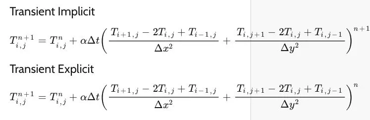
from the above Explicit formula we are going to calculate the Temperature at the each time steps. In the above formula we are define the time loop which runs 1400 time steps. Told is updated in each time loop. The initial value is also updated and also it is reinitiliaze after every iterative solvers bcoz the initial value is wash off at every iterative technquie. The initial value of RHS is assumed which gives us the assumed vlaue of T at the time step and for the next value of (i,j) T is calculated at the next time step.

In the explicit scheme there is the simple updating of the Told value from the previous or old value the solution doenot depend on the other value of T at current level and it is keep going and we got the solution simultaneously.

In the above Implicit formula there is many unknown values because we are taking up the RHS values at the time level (n+1) and there is many unknowns we have to find So we are solving this equation by some iterative solvers like Jacobi, GS and SOR.

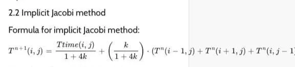
The above method is defined in a covergence loop i.e, time loop. Told value is updated in conergence loop and Tprevious values is updated in a time loop.The initilal values are assumed and the first iteration is done to calculate T at time level (n+1) which is time interval at next node. After each covergence loop the difference between previous value and T has been calculated. The error is compared to the tolerance value which has given already before that the error should not go below the tolerance value and iterations keep on going until the error value is less than the tolerance value.

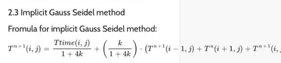
It is same as the implicit jacobi method but there is only difference that when the first iteration is done to calculate the T value and this updated T value is used to calculate the value of T at the next node.The error is compared after each convergence loop.

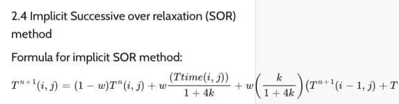
This method is used for the both jacobi and GS methods,In this method we are going to introduce a new parameter called relaxation factor(omega). It is used which over estimates the value and leads to an increase value in T for each iteration, in this way the convergence is achieved much faster than the two methods.The error is compared after each convergence loop.

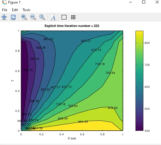
Plot for the Explicit Transient state :

:

Plots for the implicit Transient state :

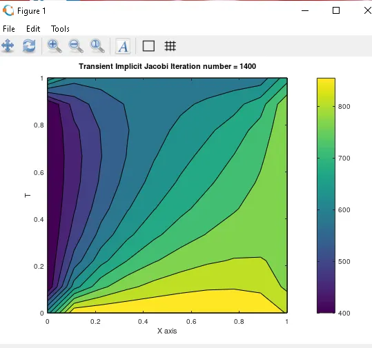
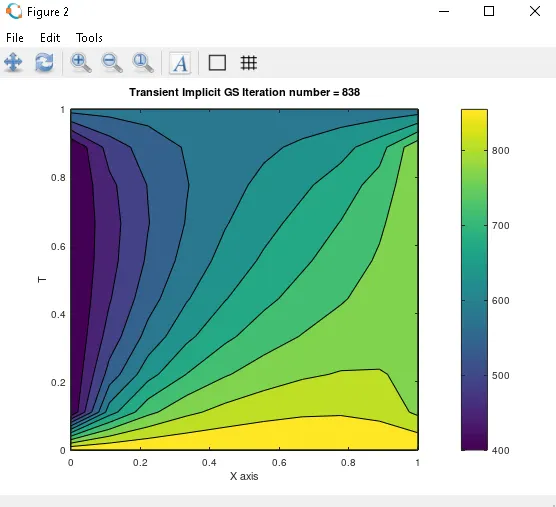
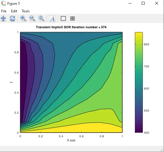
Conclusions:

• From the above graphs it is clear that explicit method is much faster to solve than the impicit method for the 2D Transient state heat conduction equation.
• From the all methods GS took least time for convergence.
• In jacobi method It tooks less time to converge the solution and SOR took more time than the GS method.
• Maximum time for convergence has given by the SOR method.
• In the transient state implicit method the iterations are less than the steady state methods because we are consider here the thermal diffiusibilty (alpha) and time interval .