Week 4.1 - Genetic Algorithm
AIM- write a code to optimize the stalagmite function and to calculate the global maxima of the functtion and explain the syntax of genetic algorithm (GA) in MATLAB
OBJECTIVE
- To write a code in MATLAB to optimize the stalagmite function and find the global maxima of the function.
- To explain the concept of genetic algorithm and syntax of GA used in programs.
- To plot the graphs of all stastical behaviour of GA and also of global maxima.
CONCEPT OF GA
GA is a way to find out the optimiation in which we study how to maximizeand minimize the partcular function and GA is a inbuilt function and it refers to basiacally minima of the particular function.
SYNTAX OF GA
EXPLANATION OF SYNTAX
x= ga( finds a local unconstrained minimum, fun,nvars)x, to the objective function, fun. nvars is the dimension (number of design variables) of fun.
x = ga( finds a local minimum fun,nvars,A,b,Aeq,beq)x to fun, subject to the linear equalities Aeq*x = beq and A*x ≤ b. (Set A=[] and b=[] if no linear inequalities exist.) ga evaluates the matrix product Aeq*x as if x is transposed (Aeq*x').
x = ga(fun,nvars,A,b,Aeq,beq,lb,ub,nonlcon)nonlcon. The function nonlcon accepts x and returns vectors C and Ceq, representing the nonlinear inequalities and equalities respectively. ga minimizes the fun such that C(x) ≤ 0 and Ceq(x) = 0. (Set lb=[] and ub=[] if no bounds exist.)
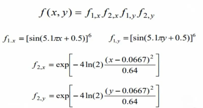
here x and y are the two variables.
PROGRAM :
for plotting a global maxima:
%program on optimise the global maxima
clear all
close all
clc

%defining our search spaces
% creating 1D array of x and y
x = linspace(0,0.6,150)
y = linspace(0,0.6,150)

%creating 2D arrays
[xx,yy] = meshgrid(x,y);

evaluate the stalagmite function
for i = 1:length(xx)
   for j = 1:length(yy)
   input_vector = xx(i,j);
   input_vector = yy(i,j);

   f(i,j) = stalagmite(input_vector);      %recalling the function
    end

end

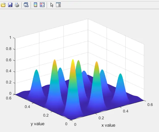
surf(xx,yy,f)
shading interp
xlabel('x value')
ylabel('y value')

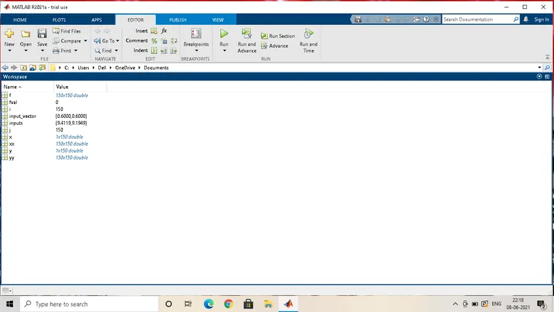
[inputs,fval] = ga(@stalagmite,2);
output
program on 3 studies
%program on optimise the stalagmite function of global maxima and study of f for maximum vs no. of iterations


clear all
close all
clc
%creating 1D array of x and y
x = linspace(0,0.6,150);
y = linspace(0,0.6,150);

num_cases = 50;             %GA runs 50 times during the program

%creating 2D array depends on x and y value
[xx,yy] = meshgrid(x,y);

%evaluating the stalagmite function
for i = 1:length(xx)
    for j = 1:length(yy)
        input_vector(1) = xx(i,j);
        input_vector(2) = yy(i,j);

        f(i,j) = stalagmite(input_vector)


    end
end

%study1 - statistical behaviour
tic

for i = 1:num_cases
    [inputs,fopt(i)] = ga(@stalagmite,2);
    xopt(i) = inputs(1)
    yopt(i) = inputs(2)

end

study1_time = toc;
%plotting
figure(1)
subplot(2,1,1)
hold on
surfc(xx,yy,f)
shading interp

plot3(xopt,yopt,fopt,'marker','o','markersize',5,'markerfacecolor','r')
title('unbounded inputs')
subplot(2,1,2)
plot(fopt)
xlabel('iterations')
ylabel('function maximum')

tic
%study 2 - statistical behaviour with upper bounds and lower bounds

for i = 1:num_cases
    [inputs,fopt(i)] = ga(@stalagmite,1,2,[],[],[],[],[0;0],[1;1]);
    xopt(i) = inputs(1)
    yopt(i) = inputs(2)

end

study2_time = toc;
%plotting
figure(2)
subplot(2,1,1)
hold on
surfc(xx,yy,f)
shading interp

plot3(xopt,yopt,fopt,'marker','o','markersize',5,'markerfacecolor','r')
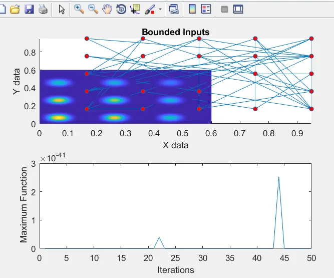
title('bounded inputs')
subplot(2,1,2)
plot(fopt)
xlabel('iterations')
ylabel('function maximum')

%study 3 increasing GA iterations
options = optimoptions('ga');
options = optimoptions(options,'populasationsize',170);

tic
for i = 1:num_cases
    [inputs,fopt(i)] = ga(@stalagmite,2,[],[],[],[],[0;0],[1;1],[],[],options);
    xopt(i) = inputs(1)
    yopt(i) = inputs(2)

end

study3_time = toc;
%plotting
figure(3)
subplot(2,1,1)
hold on
surfc(xx,yy,f)
shading interp

plot3(xopt,yopt,fopt,'marker','o','markersize',5,'markerfacecolor','r')
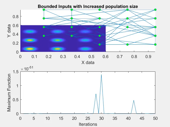
title('bounded inputs with modified population axis')
subplot(2,1,2)
plot(fopt)
xlabel('iterations')
ylabel('function maximum')
function code that is used during this program.
function [f] = stalagmite(input_vector)

x = input_vectrs(1);
y = input_vector(2);

f1 = (sin(5.1*pi.*x+0.5)).^6;
f2 = (sin(5.1*pi.*y+0.5)).^6;
f3 = exp(-4log(2).*(x-0.0667).^2/0.64);
f3 = exp(-4log(2).*(y-0.0667).^2/0.64);

f = (f1*f2*f3*f4);

end
outputs
plot1
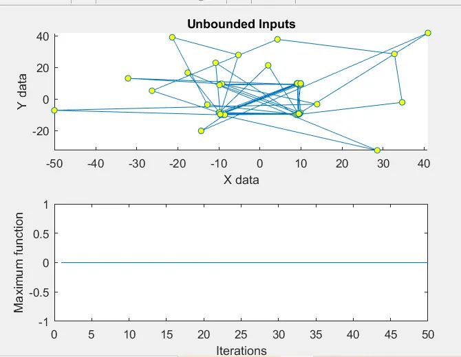
plot2
plot3
 steps
steps
errors
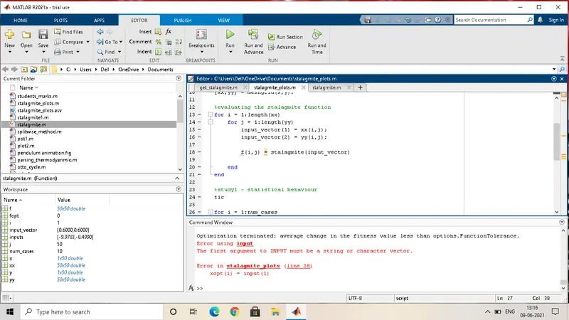
this error was show during this process it was solved by defining the inputs as inputs in the output values we got.