Week 3 - Adiabatic Flame Temperature calculation
ADIABATIC FLAME TEMPERATURE CALCULATION
AIM: To Calculate the Adiabatic Flame Temperature for constant pressure and constant volume systems under various conditions. The different conditions and the analysis to be made are mentioned below
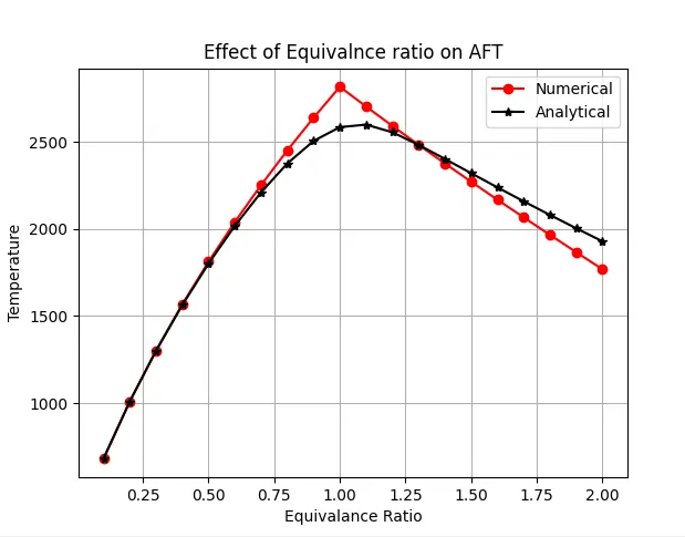
- In constant volume process, calculate the effect of equivalence ratio on AFT and plot the results
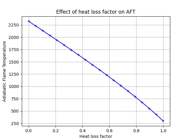
- In constant pressure process, calculate the effect of heat loss on the AFT and plot the results
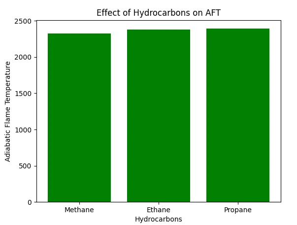
- In constant pressure process, calculate the effect of number of carbon atoms in an Alkane fuel on AFT and plot the results for 1, 2 and 3 number of carbon atoms.
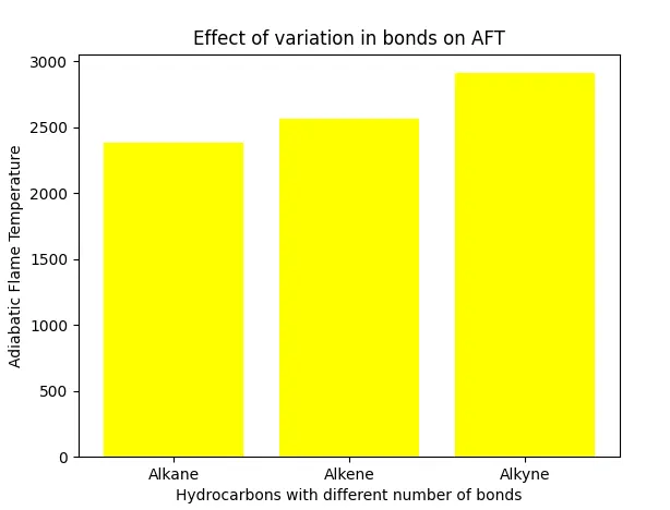
- In constant pressure process, calculate the effect of Alkane, Alkene, Alkyne double bonded fuels on AFT and plot the results.
THEORY:
A thermodynamic process is one in which the system moves from one initial state to another final stat, where both the states are in thermodynamic equilibrium. A thermodynamic process can be of constant volume, constant pressure, adiabatic and isothermal. The state of the system is defined by the values of properties like pressure, volume, internal energy, enthalpy and entropy. After a system has reached the thermodynamic equilibrium, the new state is defined by the new set of values of the thermodynamic properties.
Combustion and Its Equation:
Combustion is another word for burning. In a combustion reaction, a fuel is heated and it reacts with oxygen. The fire triangle summarizes the three things needed for combustion - a fuel, heat and oxygen. If one of these things is removed from a fire, the fire goes out. When fuels burn in combustion reactions, they release useful thermal energy (heat). Combustion reactions are used to heat our homes, power most cars, and to generate a lot of our electricity.
`C_xH_y+(x+y/4)(O_2+3.76N_2)-> xCO_2+y/2H_2O+(x+y/4)N_2`
Adiabatic Flame temperature:
In the study of combustion, there are two types of adiabatic flame temperature depending on how the process is completed: the constant volume and constant pressure. The constant volume adiabatic flame temperature is the temperature that results from a complete combustion process that occurs without any work, heat transfer or changes in kinetic or potential energy. Its temperature is higher than the constant pressure process because no energy is utilized to change the volume of the system (i.e., generate work).
INRODUCTION:
In this project AFT is calculated in constant pressure and also in constant volume conditions. In Isobaric process the difference in enthalpies of products and reactants is zero. This can be seen from the first law of thermodynamics.
Enthalpy h=U+PV where U is internal energy and PV is flow energy . In isobaric process the pressure is constant
So, h= dU + pdv + dpV
dh= dU+pdV
we know that dQ= dU + pdV
dh= dQ
As this is an insulated system so the temperature change is zero so the heat change is also zero
h1= h2
Similarly in constant volume process dQ= dU and as it is insulated system dU= 0
As it is constant volume process dv=0
Vdp = nRdT
dU= dh-nRdT
Equivalence Ratio:
It is the ratio of fuel-air ratio of current chemical reaction to the fuel-air ratio of the stoichiometric reaction
`phi = (F/A)_(current)/(F/A)_(std)`
Now based the equivalence it is said that if the ratio is less than 1 then it is called as lean mixture and if the phi value is more than 1 then the mixture is said to rich mixture.
1. AFT variation with equivalence ratio in constant volume process:
For Lean Mixture`phi<1`:
`CH_4+2/phi(O_2+3.76N_2)-> CO_2+H_2O+(2/phi-2)O_2+7.52/phiN_2`
For Rich Mixture `phi>1`:
`CH_4+2/phi(O_2+3.76N_2)->(4/phi-3) CO_2+2H_2O+(4/phi-4)CO+7.52/phiN_2`
PROGRAM:
#Effect of AFT with vaiation of Equivalance ratio

import matplotlib.pyplot as plt
import math
import numpy as np
import cantera as ct

#AFT using Python

'''
CH4 + 2 (O2+3.76N2) ---> CO2 + 2H2O + 7.52 N2
'''

def h(T,coeff):

	a1=coeff[0]
	a2=coeff[1]
	a3=coeff[2]
	a4=coeff[3]
	a5=coeff[4]
	a6=coeff[5]

	R= 8.314

	h= (a1+(a2*T/2)+(a3*pow(T,2)/3)+(a4*pow(T,3)/4)+(a5*pow(T,4)/5)+(a6/T))*R*T

	return(h)

CH4_coeff_l= [5.14987613E+00,-1.36709788E-02, 4.91800599E-05,-4.84743026E-08, 1.66693956E-11,-1.02466476E+04,-4.64130376E+00]
O2_coeff_h=[3.28253784E+00, 1.48308754E-03,-7.57966669E-07, 2.09470555E-10,-2.16717794E-14,-1.08845772E+03, 5.45323129E+00]
N2_coeff_h=[ 0.02926640E+02, 0.14879768E-02,-0.05684760E-05, 0.10097038E-09,-0.06753351E-13,-0.09227977E+04, 0.05980528E+02]
CO2_coeff_h=[3.85746029E+00, 4.41437026E-03,-2.21481404E-06, 5.23490188E-10,-4.72084164E-14,-4.87591660E+04, 2.27163806E+00]
H2O_coeff_h=[3.03399249E+00, 2.17691804E-03,-1.64072518E-07,-9.70419870E-11, 1.68200992E-14,-3.00042971E+04, 4.96677010E+00 ]
N2_coeff_l=[0.03298677E+02, 0.14082404E-02,-0.03963222E-04, 0.05641515E-07,-0.02444854E-10,-0.10208999E+04, 0.03950372E+02]
O2_coeff_l=[3.78245636E+00,-2.99673416E-03, 9.84730201E-06,-9.68129509E-09,3.24372837E-12,-1.06394356E+03, 3.65767573E+00]
CO_coeff_h=[2.71518561E+00, 2.06252743E-03,-9.98825771E-07, 2.30053008E-10,-2.03647716E-14,-1.41518724E+04, 7.81868772E+00]

R= 8.314
T_std= 298.15

def f(T,phi):

	#Enthalpy of the Reactants

	h_CH4_r= h(T_std,CH4_coeff_l)
	h_O2_r= h(T_std,O2_coeff_l)
	h_N2_r= h(T_std,N2_coeff_l)

	h_react = (phi*h_CH4_r) + 2* h_O2_r + 2*3.76*h_N2_r
	n_react = phi +2*(1+3.76)

	# Enthaply of Products

	h_CO2_p = h(T,CO2_coeff_h)
	h_O2_p= h(T,O2_coeff_h)
	h_CO_p= h(T,CO_coeff_h)
	h_N2_p= h(T,N2_coeff_h)
	h_H2O_p= h(T,H2O_coeff_h)


	if phi<= 1:
		h_prod = phi*h_CO2_p + (2*phi)*h_H2O_p + 7.52* h_N2_p+ 2*(1-phi)* h_O2_p
		n_prod = phi+ 2*phi+ 7.52+ 2*(1-phi)

	if phi>1 :
		h_prod = (4-(3*phi))* h_CO2_p + (2*phi)* h_H2O_p+ 7.52* h_N2_p+ 4*(phi-1)*h_CO_p
		n_prod= (4-(3*phi))+ 2*phi + 7.52+ 4*(phi-1)

	U_react = h_react - (n_react*R*T_std)
	U_prod= h_prod - (n_prod*R*T)

	heat = U_prod- U_react

	return heat

def fprime(T,phi):
	diff= (f(T+1e-6,phi)-f(T,phi))/(1e-6)
	return diff

tol = 1e-3
alpha= 0.2
T_guess= 1500
temp= []
phi= np.linspace(0.1,2,20)

for i in range (0,len(phi)):

	while(abs(f(T_guess,phi[i]))>tol):
		T_guess = T_guess- alpha*(f(T_guess,phi[i])/fprime(T_guess,phi[i]))
	temp.append(T_guess)
print(max(temp))


# AFT using Cantera

temp_c=[]

gas = ct.Solution('gri30.xml')

for j in range(0,len(phi)):
	n_CH4 = phi[j]
	n_O2 = 2
	n_N2 = 7.52
	gas.TPX= 298.15, 101325,{'CH4':n_CH4, 'O2': n_O2, 'N2': n_N2}
	gas.equilibrate('UV','auto')

	temp_fin = gas.T
	temp_c.append(temp_fin)

print(max(temp_c))


#plot

plt.figure(1)
plt.plot(phi,temp,'o-',color='red')
plt.plot(phi,temp_c,'*-',color='black')
plt.legend(['Numerical','Analytical'])
plt.xlabel('Equivalance Ratio')
plt.ylabel('Temperature')
plt.title('Effect of Equivalnce ratio on AFT')
plt.grid('on')
plt.show()
PLOT :
Observation:
From the baove graph we can say that the AFT value obtained using Cantera is less compared to the Python beacuse cantera accounts all the by product formations after the reactions , which results in more accurate result and more utilization energy of energy for the formation. Whereas the numerical result using python accounts for only the major elements.
On a whole in both the plots the temperature increases as Equivalance ratio gets closer to 1 and decreases when the ratio is more than 1
2. Effect of AFT with heat loss
PROGRAM:
#Effect of AFT by Variation of Heat loss


import matplotlib.pyplot as plt
import math
import numpy as np


#AFT using Python

'''
CH4 + 2 (O2+3.76N2) ---> CO2 + 2H2O + 7.52 N2
'''

def h(T,coeff):

	a1=coeff[0]
	a2=coeff[1]
	a3=coeff[2]
	a4=coeff[3]
	a5=coeff[4]
	a6=coeff[5]

	R= 8.314

	h= (a1+(a2*T/2)+(a3*pow(T,2)/3)+(a4*pow(T,3)/4)+(a5*pow(T,4)/5)+(a6/T))*R*T

	return(h)

CH4_coeff_l= [5.14987613E+00,-1.36709788E-02, 4.91800599E-05,-4.84743026E-08, 1.66693956E-11,-1.02466476E+04,-4.64130376E+00]
O2_coeff_h=[3.28253784E+00, 1.48308754E-03,-7.57966669E-07, 2.09470555E-10,-2.16717794E-14,-1.08845772E+03, 5.45323129E+00]
N2_coeff_h=[ 0.02926640E+02, 0.14879768E-02,-0.05684760E-05, 0.10097038E-09,-0.06753351E-13,-0.09227977E+04, 0.05980528E+02]
CO2_coeff_h=[3.85746029E+00, 4.41437026E-03,-2.21481404E-06, 5.23490188E-10,-4.72084164E-14,-4.87591660E+04, 2.27163806E+00]
H2O_coeff_h=[3.03399249E+00, 2.17691804E-03,-1.64072518E-07,-9.70419870E-11, 1.68200992E-14,-3.00042971E+04, 4.96677010E+00 ]
N2_coeff_l=[0.03298677E+02, 0.14082404E-02,-0.03963222E-04, 0.05641515E-07,-0.02444854E-10,-0.10208999E+04, 0.03950372E+02]
O2_coeff_l=[3.78245636E+00,-2.99673416E-03, 9.84730201E-06,-9.68129509E-09,3.24372837E-12,-1.06394356E+03, 3.65767573E+00]
CO_coeff_h=[2.71518561E+00, 2.06252743E-03,-9.98825771E-07, 2.30053008E-10,-2.03647716E-14,-1.41518724E+04, 7.81868772E+00]

R= 8.314
T_std= 298.15
Q = 802000

def f(T,H_loss):

	#Enthalpy of the Reactants

	h_CH4_r= h(T_std,CH4_coeff_l)
	h_O2_r= h(T_std,O2_coeff_l)
	h_N2_r= h(T_std,N2_coeff_l)

	h_react = h_CH4_r + 2* h_O2_r + 2*3.76*h_N2_r


	# Enthaply of Products

	h_CO2_p = h(T,CO2_coeff_h)
	h_O2_p= h(T,O2_coeff_h)
	h_CO_p= h(T,CO_coeff_h)
	h_N2_p= h(T,N2_coeff_h)
	h_H2O_p= h(T,H2O_coeff_h)

	h_prod = h_CO2_p + 2* h_H2O_p+ 7.52* h_N2_p


	heat = (h_prod -h_react)+ H_loss*Q

	return heat


def fprime(T,H_loss):
	diff= (f(T+1e-6,H_loss)-f(T,H_loss))/(1e-6)
	return diff

tol = 1e-3
alpha= 0.2
T_guess= 1500
temp= []
H_loss= np.linspace(0,1,20)

for i in range (0,len(H_loss)):

	while(abs(f(T_guess,H_loss[i]))>tol):
		T_guess = T_guess- alpha*(f(T_guess,H_loss[i])/fprime(T_guess,H_loss[i]))
	temp.append(T_guess)


#plot

plt.figure(2)
plt.plot(H_loss,temp,'+-',color='blue')
plt.xlabel('Heat loss factor')
plt.ylabel('Adiabatic Flame Temperature')
plt.title('Effect of heat loss factor on AFT')
plt.grid('on')
plt.show()
PLOT :
Obervation:
From the above graph we can observe that as heat loss factor increases the value of AFT decreases . Beacause when the system loses lot of heat through various other ways like conduction, convection or radiation etc .., the system temperature decreases.
3. Effect of AFT with respect to number of carbon atom chains:
Equations:
for Methane
CH4 + 2 (O2+3.76N2) ---> CO2 + 2H2O + 7.52 N2
for Ethane
C2H6 + 3.5(O2+3.76N2)---> 2CO2 + 3H2O + 3.5*3.76*N2
for Propane
C3H8 + 5(O2+3.76N2)----> 3CO2 + 4H20 + 5*3.76*N2
PROGRAM:
#Variation of AFT wrt to carbon atom chains

import matplotlib.pyplot as plt
import math
import numpy as np


#AFT using Python

'''
for Methane
CH4 + 2 (O2+3.76N2) ---> CO2 + 2H2O + 7.52 N2

for Ethane
C2H6 + 3.5(O2+3.76N2)---> 2CO2 + 3H2O + 3.5*3.76*N2

for Propane
C3H8 + 5(O2+3.76N2)----> 3CO2 + 4H20 + 5*3.76*N2

'''

def h(T,coeff):

	a1=coeff[0]
	a2=coeff[1]
	a3=coeff[2]
	a4=coeff[3]
	a5=coeff[4]
	a6=coeff[5]

	R= 8.314

	h= (a1+(a2*T/2)+(a3*pow(T,2)/3)+(a4*pow(T,3)/4)+(a5*pow(T,4)/5)+(a6/T))*R*T

	return(h)

CH4_coeff_l= [5.14987613E+00,-1.36709788E-02, 4.91800599E-05,-4.84743026E-08, 1.66693956E-11,-1.02466476E+04,-4.64130376E+00]
N2_coeff_h=[ 0.02926640E+02, 0.14879768E-02,-0.05684760E-05, 0.10097038E-09,-0.06753351E-13,-0.09227977E+04, 0.05980528E+02]
CO2_coeff_h=[3.85746029E+00, 4.41437026E-03,-2.21481404E-06, 5.23490188E-10,-4.72084164E-14,-4.87591660E+04, 2.27163806E+00]
H2O_coeff_h=[3.03399249E+00, 2.17691804E-03,-1.64072518E-07,-9.70419870E-11, 1.68200992E-14,-3.00042971E+04, 4.96677010E+00 ]
N2_coeff_l=[0.03298677E+02, 0.14082404E-02,-0.03963222E-04, 0.05641515E-07,-0.02444854E-10,-0.10208999E+04, 0.03950372E+02]
O2_coeff_l=[3.78245636E+00,-2.99673416E-03, 9.84730201E-06,-9.68129509E-09,3.24372837E-12,-1.06394356E+03, 3.65767573E+00]
C2H6_coeff_l=[4.29142492E+00,-5.50154270E-03, 5.99438288E-05,-7.08466285E-08, 2.68685771E-11,-1.15222055E+04, 2.66682316E+00]
C3H8_coeff_l=[0.93355381E+00, 0.26424579E-01, 0.61059727E-05,-0.21977499E-07, 0.95149253E-11,-0.13958520E+05, 0.19201691E+02]


R= 8.314
T_std= 298.15


def f(T,x):

	#Enthalpy of the Reactants

	h_CH4_r= h(T_std,CH4_coeff_l)
	h_O2_r= h(T_std,O2_coeff_l)
	h_N2_r= h(T_std,N2_coeff_l)
	h_C2H6_r=h(T_std,C2H6_coeff_l)
	h_C3H8_r= h(T_std,C3H8_coeff_l)

		# Enthaply of Products

	h_CO2_p = h(T,CO2_coeff_h)
	h_N2_p= h(T,N2_coeff_h)
	h_H2O_p= h(T,H2O_coeff_h)


	if x == 1:
		h_react_CH4 = h_CH4_r + 2* h_O2_r + 2*3.76*h_N2_r
		h_prod_CH4 = h_CO2_p + 2* h_H2O_p+ 7.52* h_N2_p

		heat = h_prod_CH4 -h_react_CH4

	if x == 2 :
		h_react_C2H6 = h_C2H6_r + 3.5*(h_O2_r + 3.76* h_N2_r)
		h_prod_C2H6 = 2* h_CO2_p + 3*h_H2O_p + 3.5*3.76* h_N2_p

		heat = h_prod_C2H6 - h_react_C2H6

	if x == 3 :
		h_react_C3H8 = h_C3H8_r + 5*(h_O2_r + 3.76* h_N2_r)
		h_prod_C3H8 = 3* h_CO2_p + 4*h_H2O_p + 5*3.76* h_N2_p

		heat = h_prod_C3H8 - h_react_C3H8


	return heat


def fprime(T,x):
	diff= (f(T+1e-6,x)-f(T,x))/(1e-6)
	return diff

tol = 1e-3
alpha= 0.2
T_guess= 1500
temp= []
x= [1, 2, 3]

for i in range (0,len(x)):

	while(abs(f(T_guess,x[i]))>tol):
		T_guess = T_guess- alpha*(f(T_guess,x[i])/fprime(T_guess,x[i]))
	temp.append(T_guess)


#plot

plt.figure(3)
plt.bar(['Methane', 'Ethane', 'Propane'],[temp[0],temp[1],temp[2]],color='green')
plt.xlabel('Hydrocarbons')
plt.ylabel('Adiabatic Flame Temperature')
plt.title('Effect of Hydrocarbons on AFT')
plt.show()
PLOT:
Observation:
The Flame temperatures are almost same and follows an ascending order of Methane , Ethane and Propane interms of temperatures because the carbon -carbon bond is stronger than carbon hydrogen bond . So apparently when the number of carbon-carbon bonds increases the energy require to break increases which inturn rises the AFT.
4. Effect of AFT wrt to Alkane , Alkene and Alkyne
Equations :
for Ethane
C2H6 + 3.5(O2+3.76N2)---> 2CO2 + 3H2O + 3.5*3.76*N2
for Ethene
C2H4 + 3(O2+3.76N2)---> 2CO2 + 2H2O + 3*3.76*N2
for Ethyne
C2H2 + 2.5(O2+3.76N2)----> 2CO2 + H20 + 2.5*3.76*N2
PROGRAM:
# Effect of AFT wrt Alkane, Alkene and Alkyne

import matplotlib.pyplot as plt
import math
import numpy as np


#AFT using Python

'''
for Ethane
C2H6 + 3.5(O2+3.76N2)---> 2CO2 + 3H2O + 3.5*3.76*N2

for Ethene
C2H4 + 3(O2+3.76N2)---> 2CO2 + 2H2O + 3*3.76*N2

for Ethyne
C2H2 + 2.5(O2+3.76N2)----> 2CO2 + H20 + 2.5*3.76*N2

'''

def h(T,coeff):

	a1=coeff[0]
	a2=coeff[1]
	a3=coeff[2]
	a4=coeff[3]
	a5=coeff[4]
	a6=coeff[5]

	R= 8.314

	h= (a1+(a2*T/2)+(a3*pow(T,2)/3)+(a4*pow(T,3)/4)+(a5*pow(T,4)/5)+(a6/T))*R*T

	return(h)

C2H6_coeff_l= [4.29142492E+00,-5.50154270E-03, 5.99438288E-05,-7.08466285E-08, 2.68685771E-11,-1.15222055E+04, 2.66682316E+00]
N2_coeff_h=[ 0.02926640E+02, 0.14879768E-02,-0.05684760E-05, 0.10097038E-09,-0.06753351E-13,-0.09227977E+04, 0.05980528E+02]
CO2_coeff_h=[3.85746029E+00, 4.41437026E-03,-2.21481404E-06, 5.23490188E-10,-4.72084164E-14,-4.87591660E+04, 2.27163806E+00]
H2O_coeff_h=[3.03399249E+00, 2.17691804E-03,-1.64072518E-07,-9.70419870E-11, 1.68200992E-14,-3.00042971E+04, 4.96677010E+00 ]
N2_coeff_l=[0.03298677E+02, 0.14082404E-02,-0.03963222E-04, 0.05641515E-07,-0.02444854E-10,-0.10208999E+04, 0.03950372E+02]
O2_coeff_l=[3.78245636E+00,-2.99673416E-03, 9.84730201E-06,-9.68129509E-09,3.24372837E-12,-1.06394356E+03, 3.65767573E+00]
C2H4_coeff_l=[3.95920148E+00,-7.57052247E-03, 5.70990292E-05,-6.91588753E-08,2.69884373E-11, 5.08977593E+03, 4.09733096E+00]
C2H2_coeff_l=[8.08681094E-01, 2.33615629E-02,-3.55171815E-05,2.80152437E-08,-8.50072974E-12, 2.64289807E+04, 1.39397051E+01 ]


R= 8.314
T_std= 298.15


def f(T,x):

	#Enthalpy of the Reactants

	h_C2H6_r= h(T_std,C2H6_coeff_l)
	h_O2_r= h(T_std,O2_coeff_l)
	h_N2_r= h(T_std,N2_coeff_l)
	h_C2H4_r=h(T_std,C2H4_coeff_l)
	h_C2H2_r= h(T_std,C2H2_coeff_l)

		# Enthaply of Products

	h_CO2_p = h(T,CO2_coeff_h)
	h_N2_p= h(T,N2_coeff_h)
	h_H2O_p= h(T,H2O_coeff_h)


	if x == 1:
		h_react_C2H6 = h_C2H6_r + 3.5*( h_O2_r + 3.76*h_N2_r)
		h_prod_C2H6 = 2*h_CO2_p + 3* h_H2O_p+ 3.5*3.76* h_N2_p

		heat = h_prod_C2H6 -h_react_C2H6

	if x == 2 :
		h_react_C2H4 = h_C2H4_r + 3*(h_O2_r + 3.76* h_N2_r)
		h_prod_C2H4 = 2* h_CO2_p + 2*h_H2O_p + 3*3.76* h_N2_p

		heat = h_prod_C2H4 - h_react_C2H4

	if x == 3 :
		h_react_C2H2 = h_C2H2_r + 2.5*(h_O2_r + 3.76* h_N2_r)
		h_prod_C2H2 = 2* h_CO2_p + h_H2O_p + 2.5*3.76* h_N2_p

		heat = h_prod_C2H2 - h_react_C2H2


	return heat


def fprime(T,x):
	diff= (f(T+1e-6,x)-f(T,x))/(1e-6)
	return diff

tol = 1e-3
alpha= 0.2
T_guess= 1500
temp= []
x= [1, 2, 3]

for i in range (0,len(x)):

	while(abs(f(T_guess,x[i]))>tol):
		T_guess = T_guess- alpha*(f(T_guess,x[i])/fprime(T_guess,x[i]))
	temp.append(T_guess)


#plot

plt.figure(4)
plt.bar(['Alkane', 'Alkene', 'Alkyne'],[temp[0],temp[1],temp[2]],color='yellow')
plt.xlabel('Hydrocarbons with different number of bonds')
plt.ylabel('Adiabatic Flame Temperature')
plt.title('Effect of variation in bonds on AFT')
plt.show()
PLOT :
Observation:
In the above case Ethane , Ethene and Ethyne are used and as we know that triple bonds are more stronger to break than double and single bonds . So it requires lot of energy to break the multiple bonds and the reflects in the above figure.
CONCLUSIONS:
1. At small values of equivalance ratio there is not much difference in AFT values , between numerical and analytical(Cantera) approach . At higher vlaues there is a significant difference.
2. AFT varies almost linearly with heat loss ,when the heat losss is more AFT is less
3. When number of carbon atoms increases in the hydrocarbons the AFT value increases
4. When number of bonds increses within the molecule which mean double or triple bond the AFT increses.