Week 3.5 - Deriving 4th order approximation of a 2nd order derivative using Taylor Table method
DERIVING 4th ORDER APPROXIMATION OF A 2nd ORDER DERIVATIVE USING TAYLOR TABLE METHOD
AIM: To write a program that derives the 4th order approximation of a 2nd order derivative using Taylor table method.
OBJECTIVES:
- Derive 4th order approximations using central difference, Skewed right sided difference, Skewed left sided difference methods.
- Prove that skewed differences are of fourth order accurate
- Compare the numerical approximations of above mentioned errors with the analytic derivative.
- Plot the errors and explain why skewed difference is useful.
THEORY:
DERIVING FOURTH ORDER APPROXIMATIONS:
Central Difference: In central difference the information from both sides of the node is considered. So for given node ‘i’ the information from i-2, i-1, i+1, i+2 are considered as this is fourth order accurate. The number of neighboring nodes that has to be taken depends upon the order of accuracy and order of derivative.
As this is 4th order accurate of a second order derivative
Order of Accuracy = stencil length – order of derivative+1 (for central difference)
Stencil length= 4+2-1 = 5
Let us consider
`(del^2u)/(delx^2)``approx` `a*f(i-2)+b*f(i-1)+c*f(i)+d*f(i+1)+e*f(i+2)`
Taylor series f(x) dx*f'(x) dx^2*f''(x) dx^3*f'''(x) dx^4*f''''(x) dx^5*f'''''(x) dx^6*f''''''(x)
stencil
a*f(i-2) a -2a 4a/2 -8a/6 16a/24 -25a/120 36a/240
b*f(i-1) b -b b/2 -b/6 b/24 -b/120 b/240
c*f(i) c 0 0 0 0 0 0
d*f(i+1) d d d/2 d/6 d/24 d/120 d/240
e*f(i+2) e 2e 4e/2 8e/6 16e/24 25e/120 36e/240
`sum` 0 0 1 0 0 ? ?
From the above table when we sum the derivatives time we get the following equations
a+b+c+d++e=0
-2a-b+0+d+2e=0
4a/2+b/2+0+d/2+4e/2=1
-8a/6-b/6+0+d/6+8e/6=0
16a/24+b/24+0+d/24+16e/24=0
The above equations has to be solved using matrix inversion method so the equation is represnted in matrix form
`[[1, 1, 1, 1, 1],[-2, -1, 0, 1, 2],[2, 1/2, 0, 1/2, 2],[-8/6, -1/6, 0, 1/6, 8/6],[16/24,1/24, 0,1/24, 16/24]]*[[a],[b],[c],[d],[e]]=[[0],[0],[1],[0],[0]]`
By solving the above matrices using AX=B , we get X matrix values
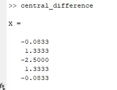
Now from the picture we can say a,b,c,d,e values are -0.0833,1.333,-2.5,1.333,-0.0833 respectively
By substituting the values of coefficients in the main equation
`(del^2u)/(delx^2)approx ((-0.0833)*f(i-2)+(1.3333)*f(i-1)+(-2.5)*f(i)+(1.3333)*f(i+1)+(-0.0833)*f(i+2))/(dx^2)+O*(dx^4)`
By solving the above equation we obtain the approximate numerical solution of the derivative.
Skewed right sided difference: In this scheme only the information from right hand sided nodes is used. For a given node ‘i’ the information from i+1, i+2,i+3,i+4, i+5 are considered as we are finding the fourth order accurate. The number of neighboring nodes that has to be taken depends upon the order of accuracy and order of derivative.
As this is 4th order accurate of a second order derivative
Order of Accuracy = stencil length – order of derivative (for skewed difference)
Stencil length= 4+2 = 6
Let us consider
`(del^2u)/(delx^2) approx a*f(i)+b*f(i+1)+c*f(i+2)+d*f(i+3)+e*f(i+4)+f*f(i+5)`
Taylor series f(x) dx*f'(x) dx^2*f''(x) dx^3*f'''(x) dx^4*f''''(x) dx^5*f'''''(x) dx^6*f''''''(x)
stencil
a*f(i) a 0 0 0 0 0 0
b*f(i+1) b b b/2 b/6 b/24 b/120 b/240
c*f(i+2) c 2c 4c/2 8c/6 16c/24 25c/120 36c/240
d*f(i+3) d 3d 9d/2 27d/6 81d/24 243d/120 729d/240
e*f(i+4) e 4e 16e/2 64e/6 256e/24 1024e/120 4096e/240
f*f(i+5) f 5f 25f/2 125f/6 625f/24 3125f/120 15625f/240
`sum` 0 0 1 0 0 0 ?
From the above table when we sum the derivatives time we get the following equations
a+b+c+d+e+f=0
0+b+2c+3d+4e+5f=0
0+b/2+2c+9d/2+16e/2+25f/2=1
0+b/6+8c/6+27d/6+64e/6+125f/6=0
0+b/24+16c/24+81d/24+256e/24+625f/24=0
0+b/120+25c/120+243d/120+1024e/120+3125f/120=0
The above equations has to be solved using matrix inversion method so the equation is represnted in matrix form
`[[1, 1, 1, 1, 1, 1] ,[0, 1, 2, 3, 4, 5],[0, 1/2, 4/2, 9/2, 16/2, 25/2] ,[0, 1/6, 8/6, 27/6, 64/6, 125/6] ,[0, 1/24, 16/24, 81/24, 256/24, 625/24],[0, 1/120, 32/120, 243/120, 1024/120, 3125/120]]*[[a],[b],[c],[d],[e],[f]]=[[0],[0],[1],[0],[0],[0]]`
By solving the above matrices using AX=B , we get X matrix values
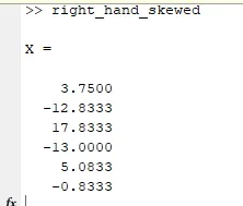
From the above picture we can say the a,b,c,d,e,f as 3.75,-12.8333,17.8333,-13,5.0833,-0.8333 respectively
By substituting the values of coefficients in the main equation
`(del^2u)/(delx^2) approx ((3.75)*f(i)+(-12.8333)*f(i+1)+(17.8333)*f(i+2)+(-13)*f(i+3)+(5.0833)*f(i+4)+(-0.8333)*f(i+5))/(dx^2)+O(dx^4)`
By solving the above equation we obtain the approximate numerical solution of the derivative.
Skewed left sided difference: In this scheme only the information from left hand sided nodes is used. For a given node ‘i’ the information from i-5, i-4,i-3,i-2, i-1 are considered as we are finding the fourth order accurate. The number of neighboring nodes that has to be taken into consideration depends upon the order of accuracy and order of derivative.
As this is 4th order accurate of a second order derivative
Order of Accuracy = stencil length – order of derivative (for skewed difference)
Stencil length= 4+2 = 6
`(del^2u)/(delx^2) approx a*f(i-5)+b*f(i-4)+c*f(i-3)+d*f(i-2)+e*f(i-1)+f*f(i)`
Taylor series f(x) dx*f'(x) dx^2*f''(x) dx^3*f'''(x) dx^4*f''''(x) dx^5*f'''''(x) dx^6*f''''''(x)
stencil
a*f(i-5) a -5a 25a/2 - 125a/6 625a/24 -3125a/120 15625a/240
b*f(i-4) b -4b 16b/2 -64b/6 256b/24 -1024b/120 4096b/240
c*f(i-3) c -3c 9c/2 -27c/6 81c/24 -243c/120 729c/240
d*f(i-2) d -2d 4d/2 -8d/6 16d/24 -32d/120 64d/240
e*f(i-1) e -e e/2 -e/6 e/24 -e/120 e/240
f*f(i) f 0 0 0 0 0 0
`sum` 0 0 1 0 0 0 ?
From the above table when we sum the derivatives time we get the following equations
a+b+c+d+e+f=0
-5a-4b-3c-2d-e+0=0
25a/2+16b/2+9c/2+4d/2+e/2=0
-125a/6-64b/6-27c/6-8d/6-e/6+0=0
625a/24+256b/24+81c/24+16d/24+e/24=0
-3125a/120-1024b/120-243c/120-32d/120-e/120=0
The above equations has to be solved using matrix inversion method so the equation is represnted in matrix form
`[[1 ,1, 1, 1, 1, 1], [ -5, -4, -3, -2, -1, 0],[ 25/2, 16/2, 9/2, 4/2, 1/2, 0], [ -125/6, -64/6, -27/6, -8/6, -1/6, 0],[ 625/24, 256/24, 81/24, 16/24, 1/24, 0],[-3125/120, -1024/20, -243/120, -32/120, -1/120, 0]]*[[a],[b],[c],[d],[e],[f]]=[[0],[0],[1],[0],[0],[0]]`
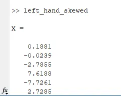
From the above picture we can say that a,b,c,d,e,f values are 0.1881,-0.0239,-2.7855,7.6188,-7.7261,2.7285 respectively
By substituting the values of coefficients in the main equation
`(del^2u)/(delx^2) approx ((0.1881)*f(i-5)+(-0.0239)*f(i-4)+(-2.7855)*f(i-3)+(7.6188)*f(i-2)+(-7.7261)*f(i-1)+(2.7285)*f(i))/(dx^2)+O*(dx^4)`
By solving the above equation we obtain the approximate numerical solution of the derivative.
PROGRAM:
Program for Error calculation using central difference method
function output = central_difference(x,dx)

% coefficent matrix for the left hand skewing method
A=[1 1 1 1 1 ;-2 -1 0 1 2 ;4/2 1/2 0 1/2 4/2 ;-8/6 -1/6 0 1/6 8/6 ;16/24 1/24 0 1/24 16/24];

% constant vector matrix
B=[0; 0; 1; 0;0 ];

% solution vector matrix
X= A\B;

% the coeffcient values
a=X(1);
b=X(2);
c=X(3);
d=X(4);
e=X(5);

% the given equation is exp(x)*cos(x)

%the second order analytical derivative is
analytical_derivative= -2*exp(x)*sin(x);

% the numerical approximation value
central_diff = (a*exp(x-2*dx)*cos(x-2*dx)+b*exp(x-dx)*cos(x-dx)+c*exp(x)*cos(x)+d*exp(x+dx)*cos(x+dx)+e*exp(x+2*dx)*cos(x+2*dx))/((dx)^2);

% the error value is stored as abs value in output variable
output=abs(analytical_derivative-central_diff);

end
Program for Error calculation using Skewed right-sided difference method
function output = right_hand_skewed(x,dx)

% coefficent matrix for the right hand skewing method
A=[1 1 1 1 1 1 ;0 1 2 3 4 5 ;0 1/2 4/2 9/2 16/2 25/2 ;0 1/6 8/6 27/6 64/6 125/6 ;0 1/24 16/24 81/24 256/24 625/24;0 1/120 32/120 243/120 1024/120 3125/120];

% constant vector matrix
B=[0; 0; 1; 0;0; 0 ];

% solution vector matrix
X= A\B;

% the coeffcient values
a=X(1);
b=X(2);
c=X(3);
d=X(4);
e=X(5);
f=X(6);

% the given equation is exp(x)*cos(x)

%the second order analytical derivative is
analytical_derivative= -2*exp(x)*sin(x);

% the numerical approximation value
right_skewed = (a*exp(x)*cos(x)+b*exp(x+dx)*cos(x+dx)+c*exp(x+2*dx)*cos(x+2*dx)+d*exp(x+3*dx)*cos(x+3*dx)+e*exp(x+4*dx)*cos(x+4*dx)+f*exp(x+5*dx)*cos(x+5*dx))/((dx)^2);

% the error value is stored as abs value in output variable
output=abs(analytical_derivative-right_skewed);

end
Program for Error calculation using Skewed left-sided difference method
function output = left_hand_skewed(x,dx)

% coefficent matrix for the left hand skewing method
A=[1 1 1 1 1 1 ; -5 -4 -3 -2 -1 0 ; 25/2 16/2 9/2 4/2 1/2 0 ; -125/6 -64/6 -27/6 -8/6 -1/6 0 ; 625/24 256/24 81/24 16/24 1/24 0;-3125/120 -1024/20 -243/120 -32/120 -1/120 0];

% constant vector matrix
B=[0; 0; 1; 0;0; 0 ];

% solution vector matrix
X= A\B;

% the coeffcient values
a=X(1);
b=X(2);
c=X(3);
d=X(4);
e=X(5);
f=X(6);

% the given equation is exp(x)*cos(x)

%the second order analytical derivative is
analytical_derivative= -2*exp(x)*sin(x);

% the numerical approximation value
left_skewed = (a*exp(x-5*dx)*cos(x-5*dx)+b*exp(x-4*dx)*cos(x-4*dx)+c*exp(x-3*dx)*cos(x-3*dx)+d*exp(x-2*dx)*cos(x-2*dx)+e*exp(x-dx)*cos(x-dx)+f*exp(x)*cos(x))/((dx)^2);

% the error value is stored as abs value in output variable
output=abs(analytical_derivative-left_skewed);

end
Main Program:
% Taylor table approximation

clear all
close all
clc

%Inputs
x=pi/3;
dx=linspace(pi/40,pi/4000,20);

%Calculation of error over range of dx

for i= 1:length(dx)
right_skewed_error(i) = right_hand_skewed(x,dx(i));  % calling the right_hand_skewed function
left_skewed_error(i)= left_hand_skewed(x,dx(i));     % calling the left_hand_skewed function
central_error(i) = central_difference(x,dx(i));      % calling the central difference function

end

%Plotting the logorthamic graphs for the errors

loglog(dx,right_skewed_error,'color','r');
hold on;
loglog(dx,left_skewed_error,'color','g');
hold on;
loglog(dx,central_error,'color','b');
title('fouth order approxs of second order derivative');                    % title is given
xlabel('dx');                                                               % x axis labelling is done
ylabel('error values');                                                     % y axis labelling is done
legend('right skewed','left skewed','central diff','location','southeast'); % legend are given for respective plots
EXPLANATION OF CODE:
1. clear all command is used to clear the workspace window
2. close all command is used to clear all the graphs, plots etc
3. clc is used to clear the command window
4. Inputs x value is given alongside dx value, which is varying from pi/40 to pi/4000 with varition of 20
5. Inorder to calculate the error at each value of dx for loop is used and the function of central difference scheme, right sided skewed, left sided skewed schemes are called.
6. Now plotting is done in log graph using loglog command where dx is in x axis and error is in y axis
7. Title, labelling and legends are given and hold on command is used to hold the previous plot.
OUTPUT:
Plot:
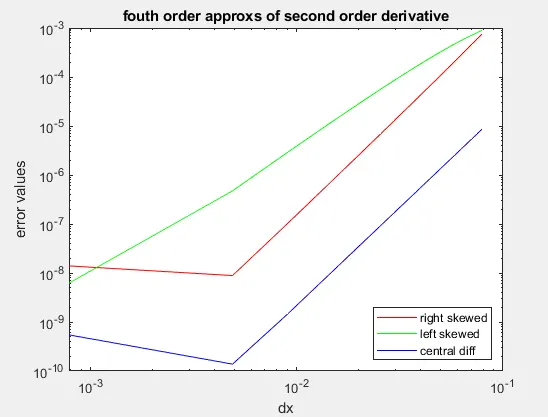
Numerical approximations of three schemes in final iteration are
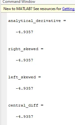
Error values in final iteration
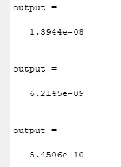
In the above picture errors are in the order right skewed, leftskewed and central difference respectively.
CONCLUSION: From the above outputs we can say the 4th order accuracy of second derivative by central difference scheme is high compared to right and left sided skewed difference schemes. Whereas , we still use right and left when there is no information on left and right respectively. For example In boundary layer condition, to one side of boundary there might no information to provide in such time we use skewed schemes.