Week 3 - Solving second order ODEs
SOLVING THE SECOND ORDER ODE
AIM: To write a program that solves the given ODE of simple pendulum with damping.
OBJECTIVES:
- To write a program to simulate the transient behavior of a simple pendulum.
- To create an animation of motion of simple pendulum using MATLAB.
INTRODUCTION:
Ordinary differential equation:
In mathematics, an ordinary differential equation is a differential equation containing one or more functions of one independent variable and the derivatives of those functions. The term ordinary is used in contrast with the term partial differential equation which may be with respect to more than one independent variable. There are different types of differential equations such as linear, non-linear, homogenous, non-homogenous etc. Based on the order of equation they are also qualified as first order differential equation if order is 1 , second order DE if the order is 2 etc. One such second order DE is given to know the transient behavior of a simple pendulum.
Simple pendulum:
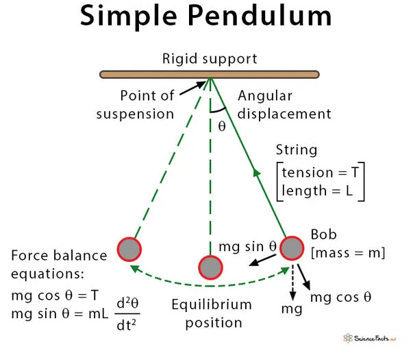
Simple pendulum known to have an object called pendulum bob hanging from the rigid support using a light wire. Initially the bob is at equilibrium, but in order to find the motion of simple pendulum the dynamic behavior of pendulum should be observed. When a bob is given a pushed a little the bob experiences a side wards force and starts oscillating to and fro with certain amplitude. The simple harmonic motion of the bob is represented by equation a shown below.
`(d^2 theta)/dt^2+g/lsintheta`= 0
Where,
`theta`= Angular displacement of pendulum bob;
g = Accelaration due to gravity in m/s^2;
l = length of the pendulum in m;
But practically, there will be drag effect and restoring forces which results in the reduction in amplitude continuously. This overall phenomenon is known as damping and the periodic motion of gradually reducing amplitude is called damped harmonic motion. The differential equation after inclusion of damping factor is given below.
`(d^2 theta)/dt^2+b/m (d theta)/dt+g/l sin theta`=0
Where,
b =damping coefficent
m= mass of the bob in kg
Now, the above second order differential equation is divided into to first order differential equations to solve easily.
Assume angular displacement `theta = theta_1`and angular velocity be
`(d theta)/dt = (d theta_1)/dt = theta_2`
`(d^2 theta)/dt^2 = (d^2 theta_1)/dt^2= d/dt((d theta_1)/dt)=(d theta_2)/dt`
Subitite the above equations in second order ODE
`(d^2theta_1)/dt^2+b/m*((d theta_1)/dt)+ g/l*sin theta_1`
`(d theta_2)/dt+b/m*theta_2+g/l*sin theta_1`
Hence we can represent them as two first order ODE
`(d theta_1)/dt = theta_2`
`(d theta_2)/dt = -b/m* theta_2-g/l*sin theta_1`
Writing these equations in matrix form
`d/dt[[theta_1],[theta_2]] = [[theta_2],[-b/m theta_2-g/l sin theta_1]]`
Where,
`theta_1`= Angular displacement of the bob
`theta_2`= Angular velocity of the bob
By solving the above equations angular displacement and angular velocity values can be calculated with respect to time.
PROGRAM:
The above equation is represented as function named ode_func
% ode function with given parameters

function[dtheta_dt]= ode_func(t,theta,b,l,g,m)
theta1=theta(1);
theta2= theta(2);
dtheta1_dt= theta2;
dtheta2_dt=-(b/m)*theta2-(g/l)*sin(theta1);
dtheta_dt=[dtheta1_dt;dtheta2_dt];
end
Main Program:
The above written function will be recalled before plotting.
The given inputs are length =1 , mass=1, b = 0.05 , and the timespan is given is 0-20 secs with initail angular displacemnt =0 and angular velocity =3 rad/sec
clear all
close all
clc
l=1;     % in meters
g=9.8;   % in m/s^2
m=1;     % in kg
b=0.05;  % damping coefficient

%intial condition
theta_i = [0;3];       % inputs ( angular displacemnt and angular velocity)

%timespace
time_space= linspace(0,20,500);  % time span range for pendulum motion

% ODE equation
[t,results]= ode45(@(t,theta)ode_func(t,theta,b,l,g,m),time_space,theta_i);

%Plotting

plot(t,results(:,1));                                                % plotting angular displacement wrt time
hold on;
plot(t,results(:,2));                                                % plotting angular velocity wrt time
axis([0 20 -4 4]);                                                   % used to fix the axis range
xlabel('Time (sec)');                                                % labelling x axis
ylabel('Angular displacement and Angular Velocity');                 % labelling y axis
title( 'Variation in Angular Displacement and Velocity wrt time and Damping effect');
legend ( 'angular displacement',' angular velocity');
pause(1);                                                            % used to pause the plot

ct=1;
for    i= 1:length(results(:,1))
    x0=0;                            % initial X-cordinate of pendulum
    y0=0;                            % initial Y-coordinate of pendulum

    x1= 1*sin(results(i,1));         % final X-cordinate of pendulum at different positions of pendulum
    y1= -1*cos(results(i,1));        % final Y-cordinate values at different positions of pendulum
% plotting
    plot([-0.5 0.5],[0 0],'linewidth',4,'color','m')  % plotting the pendulum rod
    hold on;
    plot([x0 x1],[y0 y1],'linewidth',3)               % plotting the motion of the pendulum

    plot(x1,y1,'marker','o','markersize',25,'markerfacecolor','r') % creating the pendulum bob using marker
    axis([-1.5 1.5 -1.5 0.5])                         % fixing the axis
    grid on;
    title('Motion of a simple pendulum with damping')
    pause(0.01)
       M(ct)= getframe(gcf);                          % storing each frame in M(ct)
        ct=ct+1;
        hold off;
end
% Animation of motion of pendulum
movie(M)                                                              % creating a movie
    videofile = VideoWriter('Simple_Pendulum.avi','Uncompressed AVI')  % create an empty file
    open(videofile)                                                    % open the video file
    writeVideo(videofile,M)                                            % dump the movie into the empty file
    close(videofile)

% The movie is created
Link of the output animation
https://drive.google.com/file/d/1CRvQWxHTAFyqwy-7YeCyl5cghxSBgutT/view?usp=sharing
Output Figure:
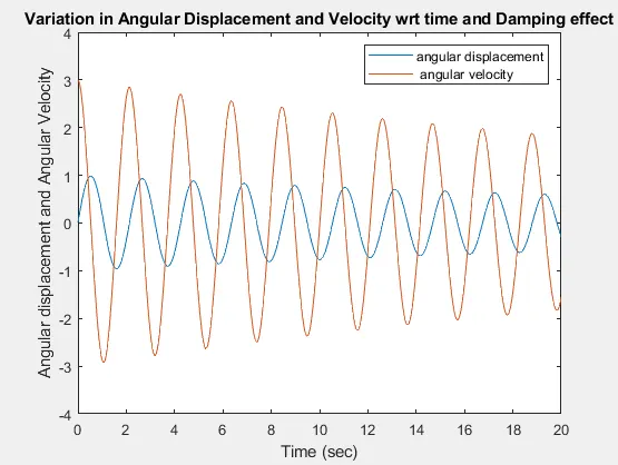
RESULTS:
1. As seen in the graph the angular displacement and velocity is decreasing alon with time thiis is due to the damping effect. It can also be said the simple harmonic motion of pendulum oscilates and finally rests at equilibrum due to this restoring forces known as damping forces , so this motion is now known as damped simple harmoinc motion .
2. From the animation it can be said that as the damping coeffiecient increases the time taken by the pendulum to reach equilibrum position decreases and viceversa.
EXPLANATION OF CODE:
1. The code starts with clear all, close all and clc
- Clear all command clears all the workspace window
- Close all command clears all the figures and graphs
- clc is used to clear the command window
2. Initail inputs l, g, m, b are entered and the initail value of angular displacement and angualr velocity is assgined to varaible theta_i
3. The time span of motion of pendulum is 0-20sec with 500 intervals in between is assigned to time_space
4. To establish the relation between all the input paramters in second order ODE a seperate function is defined named ode_func as mentioned in the above program.
5. This function ode_func is called in the main progra using ode45 command.
ode45 - ode45is an inbuilt matlab function among ode solvers. This is used to compare the 4th and 5th order differentail equations to estimate error and define step size. Where as in this instead of ode23 we used ode45 because of its accuracy in ouputs.
6. [t,results] contains the output require to plot in which results(1) contains angular displacement and results(2) contains angular velocity .
7. Using this results the angular velocity and angular displacement is plotted with respect to time.
8. Inorder to create a movie first we have to capture every frame of the motion of pendulum and for that we use a for vaiying from 1 to the lenth of angular displacement. intial and final co-ordinates are defined to plot an pendulum and capture the motion .
9. later plotting is done to ceate a rigid support and pendulum rod and to create pendulum bob, hold on command is used to visuvalize the previous frame also.
10. A title is provided and pause command is used to acheive a better animation speed.
11. Each frame is stored in M useing getframe command and later the count is increased by 1 and the loop continues.
12. After storing all the frame a videofile is created to save the movie as an uncompressed avi file .
13 Finally the movie is dumped into the file , played and after completion it closes the file.
ERRORS:
1. Error in the linewidth
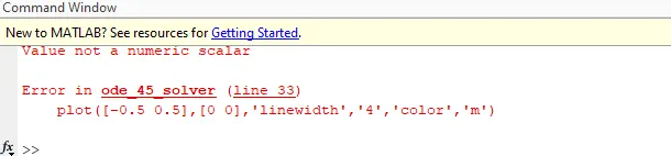
Solution- The number given for linewidth should not be quotes so after removing that the error is rectified.
2. Error in plot command

Solution: The 'P' in the plot should lower case . so after editing it the error is rectified.
3. Error in assigning variable

Solution - Intially, I have assigned variable 'y' for the output values whereas later i have chnaged to variable ' results' and forgot to change it inside the for loop after changing that the program worked .