Week 5.1 - Mid term project - Solving the steady and unsteady 2D heat conduction problem

SOLVING THE STEADY AND UNSTEADY 2D HEAT CONDUCTION PROBLEM

AIM: To write a program for solving the steady and transient 2D heat conduction problem.

OBJECTIVES:

1. To implement Jacobi, Gauss siedel and SOR methods for solving the 2D steady state heat conduction equation.
2. To implement Jacobi, Gauss siedel and SOR methods for solving the 2D transient state heat conduction equation –Implicit scheme.
3. To solve the 2D transient state heat conduction equation – Explicit scheme.
4. To plot contour between x, y and temperature.

STEADY STATE HEAT CONDUCTION: In steady state we consider that there will be no internal heat generation and convection which also implies that temperature doesn’t change with respect to time.

The general equation is

`(del^2T)/(delx^2)+(del^2T)/(dely^2)=0`

Applying Taylor series for first term of the above equation

`(del^2T)/(delx^2)= (T(i-1,j)+T(i+1,j)-2T(i,j))/(Deltax^2)`

Applying Taylor series for second term of the above equation

`(del^2T)/(dely^2)= (T(i,j-1)+T(i,j+1)-2T(i,j))/(Deltay^2)`

Summing up the equation we get

`(del^2T)/(delx^2)+(del^2T)/(dely^2)= (T(i-1,j)+T(i+1,j)-2T(i,j))/(Deltax^2) + (T(i,j-1)+T(i,j+1)-2T(i,j))/(Deltay^2)`

On further simplification,

`((Deltay^2)(T(i-1,j)+T(i+1,j)-2T(i,j)) + (Deltax^2)(T(i,j-1)+T(i,j+1)-2T(i,j)))/(Deltax^2*Deltay^2)=0`

send `T(i,j)` to other RHS side

`T(i,j)*(2*(Deltax^2+Deltay^2))/(Deltax^2*Deltay^2)=(T(i-1,j)+T(i+1,j))/(Deltax^2)+(T(i,j-1)+T(i,j+1))/(Deltay^2)`

Now consider the constant for easy calculation

`k=(2*(Deltax^2+Deltay^2))/(Deltax^2*Deltay^2)`

Upon substituting the above constant we get a final equation.

`T(i,j)=1/k*((T(i-1,j)+t(i+1,j))/(Deltax^2)+(T(i,j-1)+T(i,j+1))/(Deltay^2))`

PROGRAM:

Main Program:

clear all
close all
clc

%Inputs 

%length of domain 
L=1;

%error
error=9e9;

%tolerance 
tol=1e-4;

% number of nodes (as nx=ny=n)
n=20;

% values of x and y
x=linspace(0,1,n);
y=linspace(0,1,n);

%space between nodes 
dx=L/(n-1);
dy=L/(n-1);

% Initial Tempearture values  
T=300*ones(n,n);

%given data for tempearature at right, left, bottom and top
T_L= 400;
T_R= 800;
T_T= 600;
T_B= 900;

%Boundary conditions
T(2:n-1,1)= T_L;
T(2:n-1,n)= T_R;
T(1,2:n-1)= T_T;
T(n,2:n-1)= T_B;

%Corner points 
T(1,1)= (T_L+T_T)/2;
T(1,n)= (T_T+T_R)/2;
T(n,1)=(T_L+T_B)/2;
T(n,n)=(T_B+T_R)/2;

Told=T;

% Value of k 
k= 2*(dx^2+dy^2)/(dx^2*dy^2);

% calling the functions
jacobi_steady(T,Told,n,error,tol,x,y,dx,dy,k);
gauss_steady(T,Told,n,error,tol,x,y,dx,dy,k);
SOR_steady(T,Told,n,error,tol,x,y,dx,dy,k);

Jacobi method:

Jacobi iterative method is considered as an iterative algorithm which is used for determining the solutions for the system of linear equations in numerical linear algebra, which is diagonally dominant. In this method, an approximate value is filled in for each diagonal element. Until it converges, the process is iterated.

`x^(k+1)=[D]^-1(b-(L+U)x^k)`

where L - Lower diagonal Matrix and U- upper diagonal Matrix

D- Diagonal Matrix

function[]= jacobi_steady(T,Told,n,error,tol,x,y,dx,dy,k)

% meshgrid is used to create a 2D domain
[X,Y]=meshgrid(x,y);

% JACOBI 

% iteration count 
    jac_iter = 1;      

while (error>tol)
    % space loop 
     for i=2:n-1          
        for j=2:n-1
            T(i,j)= (1/k)*((Told(i-1,j)+Told(i+1,j))/dx^2 + (Told(i,j-1)+Told(i,j+1))/dy^2);
        end
    end
    error= max(max(abs(Told-T))); % max(max(T)) to convert from 2D array to a scalar
    jac_iter = jac_iter + 1;
    Told=T;    

end
% figure is plotted 
figure(1)
contourf(X,Y,T,'ShowText','ON');                        % showtext is used to vizuvalise the values of tempeartures 
title({['JACOBI ITERATIONS = ',num2str(jac_iter)]}); 
xlabel('X AXIS');                                       % xaxis labelling 
ylabel('Y AXIS');                                       % yaxis labelling  
colormap(jet);                                          % jet mode is on 
colorbar;                                               % color bar is used to represent the ranges of temp 
set(gca,'Ydir','reverse');                              % this command is used to reverse the y axis limits 

end

Gauss-Siedel method:

The Gauss-Seidel method is a technique for solving the equations of the linear system of equations one at a time in sequence, and uses previously computed results as soon as they are available.

`L*x^(k+1)=b-U*x^k`

function[]= gauss_steady(T,Told,n,error,tol,x,y,dx,dy,k)

% to create a 2D domain
[X,Y]=meshgrid(x,y);

% GS

%iteration count  
  gs_iter = 1;
while (error>tol)
    % space loop
     for i=2:n-1
        for j=2:n-1
            T(i,j)= (1/k)*((T(i-1,j)+Told(i+1,j))/dx^2 + (T(i,j-1)+Told(i,j+1))/dy^2); %Uses current T values for Left and Top nodes
        end
    end
    error= max(max(abs(Told-T))); % max(max(T)) to convert from 2D array to a scalar
    gs_iter = gs_iter + 1;        % count is increased by one 
    Told=T;

end

% Figure is plotted 
figure(2)
contourf(X,Y,T,'ShowText','ON');                % Show txt is on to represnt the tempearture values in the figure
colormap(jet);
colorbar;                                       % Using to represent different colors  
set(gca,'Ydir','reverse')                       % used to reverse the axis limits of y axis 
title({['GS ITERATIONS = ',num2str(gs_iter)]}); % Title is given 
xlabel('X AXIS');                               % xaxis labelling 
ylabel('Y AXIS');                               % yaxis labelling 
end

SOR Method:

The successive over relaxation method (SOR) is a method of solving a linear system of equations derived by extrapolating the Gauss-Seidel method. This extrapolation takes the form of a weighted average between the previous iterate and the computed Gauss-Seidel iterate successively for each component.

`x^(k+1)=(1-omega)x^k+omega*M^-1(b-U*x^k)`

`M=L+D`

L,D are the diagonal matrix

when omega is greater than 1 to certain extent the solution converges .

When omega is less than 1 the solution converges slowly, it is also called as sucessive under relaxation.This is genearlly used for non-linear equations.

function[]= SOR_steady(T,Told,n,error,tol,x,y,dx,dy,k)

% to create 2D domain 
[X,Y]=meshgrid(x,y);

% SOR
% iteration count 
  sor_iter = 1;
  
  % relaxation factor 
  omega = 1.2;
  
while (error>tol)
    % space loop 
     for i=2:n-1
        for j=2:n-1
            T_GS = (1/k)*((T(i-1,j)+Told(i+1,j))/dx^2 + (T(i,j-1)+Told(i,j+1))/dy^2); %Uses current T values for Left and Top nodes
            T(i,j) = (1-omega)*Told(i,j) + omega*T_GS; 
        end
    end
    error= max(max(abs(Told-T))); % max(max(T)) to convert from 2D array to a scalar
    sor_iter = sor_iter + 1;
    Told=T;

end

% figure is plotted 
figure(3)
contourf(X,Y,T,'ShowText','ON');           % Showtext is on to represent the value of temepeartures 
colormap(jet);                              
colorbar;                                  % colorbar is used to represent the range of colors 
set(gca,'Ydir','reverse')                  % this command is used to reverse the y axis limits
title({['SOR ITERATIONS = ',num2str(sor_iter)]}); 
xlabel('X AXIS');                          % xaxis labelling
ylabel('Y AXIS');                          % yaxis labelling
end

OUTPUTS:

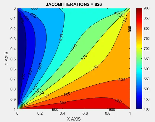
steady state jacob method

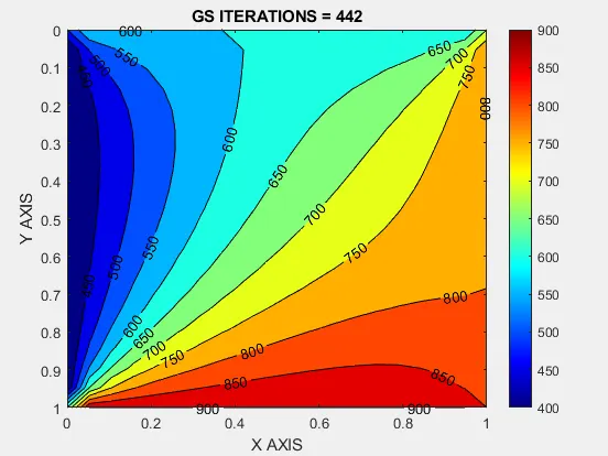
steady state gauss-sidel method

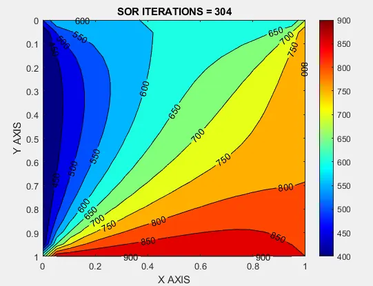
steady state sor method

CONCLUSION:

From the above figures we can say that the number iterations required for by gauss siedel is 442 which lesser than jacobi method because we are using the updated values in the equation for gauss method. In the similar way the number iterations required for SOR method to converge (304) is less than gauss sidel method as we are using an over relaxation factor in order to converge faster. So SOR method is effecient comapred to the other two processes.

Observation: In SOR method the solution converges upto omega=1.5 after that the solution starts to diverge.

TRANSIENT STATE HEAT CONDUCTION :

In transient state heat conduction, temperature changes with respect to time. Here time marching solution plays an important role in this solution. This can be solved in two method

1. Explicit
2. Implicit

Assuming that there is no convection and no internal heat generation

The general equation of transient state 2D heat conduction

`(delT)/(delt)+alpha*((del^2T)/(delx^2)+(del^2T)/(dely^2))=0`

Explicit Scheme:

In this scheme, all the information is taken from previous step to solve the next time step.

`(T^(n+1)(i,j)-T^n(i,j))/(Deltat)=alpha*((T(i-1,j)+T(i+1,j)-2*T(i,j))/(Deltax^2)+(T(i,j-1)+T(i,j+1)-2*T(i,j))/(Deltay^2))^n`

Let us consider constants for simple calculations

`k1=alpha*(Deltat)/(Deltax^2)`

`k2=alpha*(Deltat)/(Deltay^2)`

Substitutes the constants in the equation

`T^(n+1)(i,j)=T^n(i,j)+k1*(T(i-1,j)+T(i+1,j)-2*T(i,j))+k2*(T(i,j-1)+T(i,j+1)-2*T(i,j))`

Here stability factors comes into play

We know that CFL constant values should less than or equal for the solution to be stable

So`k1+k2le0.5`

Which implies that dt value should be considered accordingly.

CFL CONDITION: Generally, the CFL condition expresses that the time step length with in the mesh should be lower than the distance between the mesh elements.

Main program:

clear all
close all
clc

%Inputs 

%thermal diffusivity
alpha=1.4;

%length of domain 
L=1;

% time step 
dt=4e-4;

%error
error=9e9;

%tolerance 
tol=1e-4;

% number of nodes (as nx=ny=n)
n=20;

% values of x and y
x=linspace(0,1,n);
y=linspace(0,1,n);

%space between nodes 
dx=L/(n-1);
dy=L/(n-1);

% Initial Tempearture values  
T=300*ones(n,n);

%given data for tempearature at right, left, bottom and top
T_L= 400;
T_R= 800;
T_T= 600;
T_B= 900;

%Boundary conditions
T(2:n-1,1)= T_L;
T(2:n-1,n)= T_R;
T(1,2:n-1)= T_T;
T(n,2:n-1)= T_B;

%Corner points 
T(1,1)= (T_L+T_T)/2;
T(1,n)= (T_T+T_R)/2;
T(n,1)=(T_L+T_B)/2;
T(n,n)=(T_B+T_R)/2;

% To create 2D domain 
[X,Y]=meshgrid(x,y);

% Intial condition for the tempearture profile
Told=T;

% Constant values 
k1=(alpha*dt)/(dx^2);
k2=(alpha*dt)/(dy^2);

% CFL condition 
CFL=k1+k2;
%dt= 0.5*(dx^2*dy^2)/(alpha*(dx^2+dy^2));
% dt value should be equal to less than 4.9e-4 so the  from above equation , so value of dt is
% taken as 4e-4 in the input 

% iteration count 
unsteady_itr=1;


        while (error>tol)
        % space loop 
        for i=2:n-1
        for j=2:n-1
            term1=Told(i,j);
            term2=Told(i-1,j)-2*Told(i,j)+Told(i+1,j);
            term3=Told(i,j-1)-2*Told(i,j)+Told(i,j+1);
            T(i,j)=term1+(k1*(term2))+(k2*(term3));
        end 
        end
    error= max(max(abs(Told-T))); % max(max(T)) to convert from 2D array to a scalar
    Told=T;
    unsteady_itr= unsteady_itr + 1;  
        end
  
   
figure(4)
contourf(X,Y,T,'ShowText','ON');  % showtext is on to represent the tempearture values 
title({['TRANSIENT EXPLICIT ITERATIONS = ',num2str(unsteady_itr)]}); 
xlabel('X AXIS');                 % xaxis labelling 
ylabel('Y AXIS');                 % yaxis labelling 
colormap(jet);                    % colormap mode is set to jet 
colorbar;                         % color bar to used differentiate the temperature ranges  
set(gca,'Ydir','reverse');        % this statement is used to reverse the yaxis limits 

OUTPUT:

transient explicit method

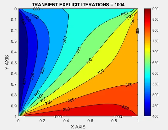
CONCLUSION: In the above figure there is no need for converging a solution as we know the values at given time step. So the total time iterations the function ran for the solution is 1004.

Implicit Scheme:

In this Scheme the information is taken from domain, so the solution doesn’t require any stability conditions.

The general equation for implicit heat conduction method is

`(T^(n+1)(i,j)-T^n(i,j))/(Deltat)=alpha*((T(i-1,j)+T(i+1,j)-2*T(i,j))/(Deltax^2)+(T(i,j-1)+T(i,j+1)-2*T(i,j))/(Deltay^2))^(n+1)`

For easy simplification we consider constants

`k1=alpha*(Deltat)/(Deltax^2)`

`k2=alpha*(Deltat)/(Deltay^2)`

Using the constants in above equation

`T^(n+1)(i,j)=(1+2*k1+2*k2)^-1*(T^n(i,j)+k1*(T(i-1,j)+T(i+1,j)-2*T(i,j))+k2*(T(i,j-1)+T(i,j+1)-2*T(i,j)))`

Here the iterative solvers are used because we don’t know the information in n+1 th step .

Main Program:

clear all
close all
clc

%Inputs 

%thermal diffusivity
alpha=1.4;

%length of domain 
L=1;

%error
error2=9e9;

%tolerance 
tol=1e-4;

% number of nodes (as nx=ny=n)
n=20;

%number of timesteps 
dt=4e-4;

% values of x and y
x=linspace(0,1,n);
y=linspace(0,1,n);

%space between nodes 
dx=L/(n-1);
dy=L/(n-1);

% Initial Tempearture values  
T=300*ones(n,n);

%given data for tempearature at right, left, bottom and top
T_L= 400;
T_R= 800;
T_T= 600;
T_B= 900;

%Boundary conditions
T(2:n-1,1)= T_L;
T(2:n-1,n)= T_R;
T(1,2:n-1)= T_T;
T(n,2:n-1)= T_B;

%Corner points 
T(1,1)= (T_L+T_T)/2;
T(1,n)= (T_T+T_R)/2;
T(n,1)=(T_L+T_B)/2;
T(n,n)=(T_B+T_R)/2;

% Intial values of temperature profiles 
Told=T;
T_prev=Told;

%Constant values 
k1=(alpha*dt)/(dx^2);
k2=(alpha*dt)/(dy^2);

% to create a 2D domain
%[X,Y]=meshgrid(x,y);

% Calling the functions 
jacobi_transient(T,Told,T_prev,n,error2,tol,x,y,k1,k2);
guass_transient(T,Told,T_prev,n,error2,tol,x,y,k1,k2);
SOR_transient(T,Told,T_prev,n,error2,tol,x,y,k1,k2);

Jacobian Method :

function[]=jacobi_transient(T,Told,T_prev,n,error2,tol,x,y,k1,k2)

% To create 2D domain 
[X,Y]=meshgrid(x,y);

% space and time iterations 
jac_trans=1;
jac_trans_time=1;

%time loop 
while (error2>tol)
    %Reinitilization of error
  error1 = 9e9;
  %space loop
    while(error1>tol)
     for i=2:n-1
        for j=2:n-1
            term1=(1+2*k1+2*k2)^(-1);
            term2=k1*term1;
            term3=k2*term1;
            H=(Told(i-1,j)+Told(i+1,j));
            V=(Told(i,j-1)+Told(i,j+1));
            T(i,j)=(T_prev(i,j)*term1+H*term2+V*term3);
        end
     end
      error1= max(max(abs(Told-T))); % max(max(T)) to convert from 2D array to a scalar
      Told=T;
      jac_trans= jac_trans + 1;

    end
    error2=max(max(abs(T_prev-T)));% max(max(T)) to convert from 2D array to a scalar
    T_prev=T;
    jac_trans_time=jac_trans_time+1;
end

%Figure
figure(5)
contourf(X,Y,T,'ShowText','ON');  % Showtext is on to represent the values of tempearture 
title({['TRANSIENT JAC-IMPLICT ITERATIONS = ',num2str(jac_trans)]});
xlabel('X AXIS');                 % xaxis labelling 
ylabel('Y AXIS');                 % yaxis labelling 
colormap(jet);                    % jet mode is on for color map 
colorbar;                         % color bar is to identify different tempearture zones 
set(gca,'Ydir','reverse');        % this statement is used to reverse the y axis limits

end

Guass-Siedel Method:

function[]=guass_transient(T,Told,T_prev,n,error2,tol,x,y,k1,k2)

% To create 2D domain 
[X,Y]=meshgrid(x,y);

% space and time iterations 
gauss_trans=1;
gauss_trans_time=1;

%time loop 
while (error2>tol)
    %Reinitilization of error
  error1 = 9e9;
   %space loop
    while(error1>tol)
     for i=2:n-1
        for j=2:n-1
            term1=(1+2*k1+2*k2)^-1;
            term2=k1*term1;
            term3=k2*term1;
            H=(T(i-1,j)+Told(i+1,j));
            V=(T(i,j-1)+Told(i,j+1));
            T(i,j)=(T_prev(i,j)*term1+H*term2+V*term3);
        end
     end
      error1= max(max(abs(Told-T))); % max(max(T)) to convert from 2D array to a scalar
      Told=T;
      gauss_trans= gauss_trans + 1;

    end
    error2=max(max(abs(T_prev-T))); % max(max(T)) to convert from 2D array to a scalar
    T_prev=T;
    gauss_trans_time=gauss_trans_time+1;
end

%Figure
figure(6)
contourf(X,Y,T,'ShowText','ON');  % Showtext is on to represent the values of tempearture 
title({['TRANSIENT GS-IMPLICT ITERATIONS = ',num2str(gauss_trans)]});
xlabel('X AXIS');                 % xaxis labelling 
ylabel('Y AXIS');                 % yaxis labelling 
colormap(jet);                    % jet mode is on for color map 
colorbar;                         % color bar is to identify different tempearture zones 
set(gca,'Ydir','reverse');        % this statement is used to reverse the y axis limits

end

SOR Transient Method:

function[]=SOR_transient(T,Told,T_prev,n,error2,tol,x,y,k1,k2)

% To create 2D domain 
[X,Y]=meshgrid(x,y);

% relaxation factor
omega=1.2;

% space and time iterations 
SOR_trans=1;
SOR_trans_time=1;

%time loop 
while (error2>tol)
    %Reinitilization of error
  error1 = 9e9;
   %space loop
    while(error1>tol)
     for i=2:n-1
        for j=2:n-1
            term1=(1+2*k1+2*k2)^(-1);
            term2=k1*term1;
            term3=k2*term1;
            H=(T(i-1,j)+Told(i+1,j));
            V=(T(i,j-1)+Told(i,j+1));
            T(i,j)=(T_prev(i,j)*term1+H*term2+V*term3);
            T(i,j)=(1-omega)*(Told(i,j))+omega*(T(i,j));
        end
     end
      error1= max(max(abs(Told-T))); % max(max(T)) to convert from 2D array to a scalar
      Told=T;
      SOR_trans= SOR_trans + 1;

    end
    error2=max(max(abs(T_prev-T))); % max(max(T)) to convert from 2D array to a scalar
    T_prev=T;
    SOR_trans_time=SOR_trans_time+1;
end

%Figure
figure(7)
contourf(X,Y,T,'ShowText','ON');  % Showtext is on to represent the values of tempearture 
title({['TRANSIENT SOR-IMPLICT ITERATIONS = ',num2str(SOR_trans)]}); 
xlabel('X AXIS');                 % xaxis labelling 
ylabel('Y AXIS');                 % yaxis labelling 
colormap(jet);                    % jet mode is on for color map 
colorbar;                         % color bar is to identify different tempearture zones 
set(gca,'Ydir','reverse');        % this statement is used to reverse the y axis limits
end

EXPLANANTION OF CODE ( FOR ALL THE ABOVE WRITTEN PROGRAM):

1. clear all command clears all the memory of worspace window.

2. close all is used to clear the graphs plots etc

3. clc is used to clear the command window

4. Inputs were given

5. In main prgrams the functions were called.

6. In functions while loops were written and counting was done in order to know the number of iterations the method takes to converge i.e, for jacobi, gauss-siedel, SOR methods

7. In Steady state function there is no time loop where in transient functions time loops are used. Epescially in transient implicit function time and space loop are utilized.

8. mesh grid command is used to create a 2D domain and that is used along with tempearture to plot a contour.

9. The contours are colored and temperature values are represented accordingly.

10. Title, axis labelling is done

11. set command is used to reverse the yaxis limits.

12. Detalied explanation is given in the program itself.

OUTPUTS:

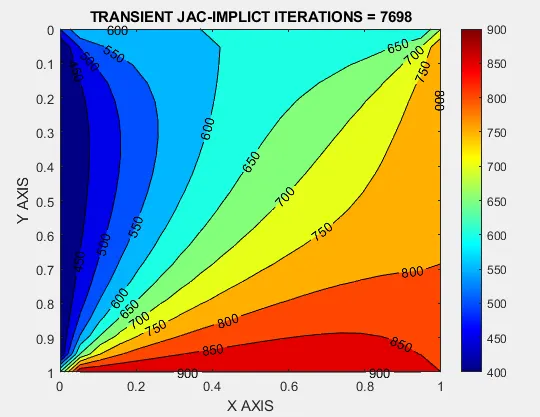
transient implicit jacob method

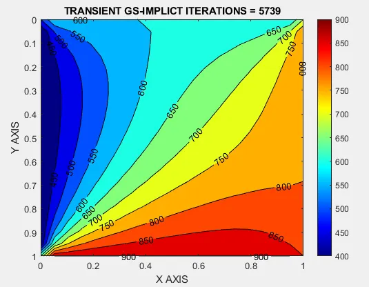
transient implicit gauss-siedel method

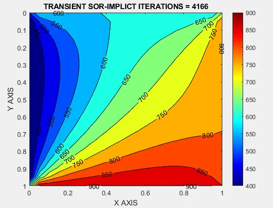
transient implicit sor method

CONCLUSION:

From the above figures we can say that the number iterations required for by gauss siedel is 5739 which lesser than jacobi method because we are using the updated values in the equation for gauss method. In the similar way the number iterations required for SOR method to converge (4166) is less than gauss sidel method as we are using an over relaxation factor in order to converge faster . If we use under relaxation even the solution converges but slowly. So SOR method is effecient comapred to the other two methods.

Observation: In SOR method the solution converges upto omega=1.5 after that the solution starts to diverge.