Week 3 - Adiabatic Flame Temperature calculation

1. Adiabatic flame temperature variation with Equivalence ratio (In constant volume-chamber):

Equivalence ration, `phi` is defined as ratio of actual fuel-air ratio to stoichiometric fuel-air ratio

`phi = (F//A)/(F//A)_(st)`

Combustion of methane with air in stoichiometric conditions is represented by following equation

`CH_4 + 2(O_2 + 3.76N_2 ) -> CO_2 + 2H_2O + 7.52N_2`, when `phi = 1`

For combustion of methane in lean mixture, excess nitrogen and oxygen are added to the products side and is represented by

`CH_4 + 2/phi(O_2 + 3.76N_2 ) -> CO_2 + 2H_2O + 7.52/phiN_2+ (2/phi-2)O_2`, when `phi < 1`

For combustion of methane in rich mixture, insufficient oxygen for combustion will lead to formation of CO and is represented by

`CH_4 + 2/phi(O_2 + 3.76N_2 ) -> (4/phi-3)CO_2 + 2H_2O + 7.52/phiN_2+ (4-4/phi)CO`, when `phi > 1`

In a constant volume combustion, the internal energy of the system is constant, meaning the reactants and products have same internal energy.

The change in internal energy is hence 0. Using first of thermodynamics,

`dU = dQ - W = 0`

Change in enthalpy is

`dH = dU + Delta(PV)` ==> `dH = dU + PDeltaV + VDeltaP`

Since `dU = DeltaV = 0` for constant volume process,

`dH - VDeltaP = 0` ==> `H_p - H_r - V(P_p-P_r) = 0`

where, subscript p -> products and r -> reactants.

Using ideal gas equation, `PV = nRT`,

`H_p -H_r - R(N_pT_(ad)-N_rT_i) = 0`

where `T_i` -> initial temperature and `T_(ad)` -> adiabatic flame temperature

Solving for `T_(ad)` using a computer program can be done using Newton Raphson method on above equation.

`H_r` and `H_p` of combustion can be calculated for the chemical equations based on `phi` value as a f(T) using following relation

`H/(RT) = a1 + a_2T/2 + a_3T^2/3 + a_4T^3/4+a_5T^4/5+a_6/T`

where the constants `a_1` to `a_6` can be obtained from NASA's thermodynamic data

With R and `T_i` known, `T_(ad)` can be found by assuming an initial value and using Newton Raphson iterative method to converge on exact result. An array of values are taken for phi between 0.5 and 1.5 at an interval of 0.05. For each value of phi, adiabatic flame temperature is calcuated.

The same problem is then solved using equilibrate method in cantera library. Temperature, pressure and mole-fraction of reactants are provided to cantera using TPX. The system is then solved by maintaining internal energy and specific volume constant by passing the 'UV' argument to equilibrate method. Adiabatic flame temperature is then obtained for different phi values. Both the results are plotted against phi.

The python program to solve methane combusiton in constant volume using Newton-Raphson method and Cantera is shown below

"""
Calculation of adabatic flame temperature for combustion of CH4 in constant volume
using NASA's thermodynamic data for vairous equivalence ratio
"""
import numpy as np
import matplotlib.pyplot as plt
import cantera as ct


## Using Newton Raphson method in Python
# Constants and inputs
R = 8.314			# Universal gas constant
Ti = 298.15			# Initial temperature
alpha = 0.7			# Under-relaxation factor
T_init = 1500		# Initial guess value for adiabatic flame temperature
tol = 1e-3			# Tolerance for convergence of T_adiabatic
phi_arr = np.linspace(0.5,1.5,21)		# Equivalence ratio array
T_ad = []			# Result array - python
T_ad_ct = []		# Result array - cantera
counter_arr = []	# iteration counter array

# NASA thermodynamic data
# reactants
ch4_coeff_l = [5.14987613E+00, -1.36709788E-02, 4.91800599E-05, -4.84743026E-08, 1.66693956E-11, -1.02466476E+04, -4.64130376E+00]
o2_coeff_l = [3.78245636E+00, -2.99673416E-03, 9.84730201E-06, -9.68129509E-09, 3.24372837E-12, -1.06394356E+03, 3.65767573E+00]
n2_coeff_l = [0.03298677E+02, 0.14082404E-02, -0.03963222E-04, 0.05641515E-07, -0.02444854E-10, -0.10208999E+04, 0.03950372E+02]
# products
co2_coeff_h = [3.85746029E+00, 4.41437026E-03, -2.21481404E-06, 5.23490188E-10, -4.72084164E-14, -4.87591660E+04, 2.27163806E+00]
h2o_coeff_h = [3.03399249E+00, 2.17691804E-03, -1.64072518E-07, -9.70419870E-11, 1.68200992E-14, -3.00042971E+04, 4.96677010E+00]
n2_coeff_h = [0.02926640E+02, 0.14879768E-02, -0.05684760E-05, 0.10097038E-09, -0.06753351E-13, -0.09227977E+04, 0.05980528E+02]
o2_coeff_h = [3.28253784E+00, 1.48308754E-03, -7.57966669E-07, 2.09470555E-10, -2.16717794E-14, -1.08845772E+03, 5.45323129E+00]
co_coeff_h = [2.71518561E+00, 2.06252743E-03, -9.98825771E-07, 2.30053008E-10, -2.03647716E-14,  -1.41518724E+04, 7.81868772E+00]

# calculate heat of formation based on temperature and thermodynamic coeffs
def h(T,coeffs):
	# H = (a1 + a2*T/2 + a3*T^2/3 + a4*T^3/4 + a5*T^4/5 + a6/T) * R * T
	return (coeffs[0] + coeffs[1]*T/2 + coeffs[2]*pow(T,2)/3 + coeffs[3]*pow(T,3)/4 + coeffs[4]*pow(T,4)/5 + coeffs[5]/T) * T * R

# Solve enthalpy balance equation and return the residual
def f(T,phi):
	# Hp - Hr - R(NpT(ad)-NrTi) = 0
	h_r = h(Ti,ch4_coeff_l) + (2/phi) * ( 2*h(Ti,o2_coeff_l) + 3.76*h(Ti,n2_coeff_l))
	n_r = 1 + 2/phi*(1+3.76)
	if phi <= 1:
		# CH4 + 2/phi*(O2 + 3.76N2 ) -> CO2 + 2H2O + 7.52/phi N2 + (2/phi-2) O2,			when phi <= 1	
		h_p = h(T,co2_coeff_h) + 2*h(T,h2o_coeff_h) + 7.52/phi*h(T,n2_coeff_h) + (2/phi - 2)*h(T,o2_coeff_h)
		n_p = 1 + 2 + 7.52/phi + (2/phi - 2)
	else:
		# CH4 + 2/phi(O2 + 3.76N2 ) -> (4/phi-3)CO2 + 2H2O + 7.52/phi N2 + (4-4/phi) CO,	when phi > 1
		h_p = (4/phi-3)*h(T,co2_coeff_h) + 2*h(T,h2o_coeff_h) + 7.52/phi*h(T,n2_coeff_h) + (4 - 4/phi)*h(T,co_coeff_h)
		n_p = (4/phi - 3) + 2 + 7.52/phi + (4 - 4/phi)
	return h_p - h_r - R*(n_p*T - n_r*Ti)

# calculate derivative of f(T) using numerical first order Taylor series method
def fprime(T,phi):
	return (f(T+1e-6,phi) - f(T,phi))/1e-6

# Solve for T_adiabatic for given values of phi
for phi in phi_arr:
	T = T_init				# initialize adiabatic temperature
	counter = 0 					# iteration counter
	f_T = f(T,phi)
	while abs(f_T) > tol:
		T = T - alpha*(f_T/fprime(T,phi))
		counter += 1
		f_T = f(T,phi)
		if counter > 1000:
			break
	T_ad.append(T)
	counter_arr.append(counter)

# plot the results
plt.plot(phi_arr,T_ad,"-*",color="red",label="Python")
plt.title("Adiabatic flame temperature vs Equivalence ratio")
plt.xlabel("Equivalence ratio")
plt.ylabel("Adiabatic flame temperature [K]")


## Using Cantera 
for phi in phi_arr:
	gas = ct.Solution("gri30.xml")
	gas.TPX = 298.15, 101325, {'CH4':1,'O2':2/phi,'N2':7.52/phi}
	gas.equilibrate('UV')
	T_ad_ct.append(gas.T)

# plot the results
plt.plot(phi_arr,T_ad_ct,"-*",color="blue",label="Cantera")
plt.legend()
plt.show()

Result:

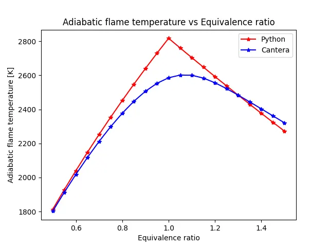
For small values of `phi` both the methods predict same adiabatic flame temperature. `T_(ad)` is maximum at `phi=1` for both the methods. However, Cantera predicts lower value for temperature compared to Newton-Raphson method. For larger values of `phi`, the temperature drops sharply for Newton-Raphson method that reaches below Cantera prediction at a value of 1.5 for `phi`.

This difference in result is because, Cantera includes much more number of speicies in the equation to solve enthalpy balance compared to our manual technique. The heat of formation of the ignored species and their increase in sensible enthalpy contribute to the difference in enthalpy balance and hence the adiabatic flame temperature. Except for the condition of very rich fuel combustion, the effect of these additional species would reduce the adiabatic flame temperatures.

2. Flame temperature variation with Heat loss (In constant pressure-chamber) :

From first law of thermodynamics

`dU = dQ - PDeltaV`

where dQ is defined as

`dQ = "H_loss_factor" * dQ_(max)`, for `0 <="H_loss_factor"<=1`

`dQ_(max)` is given as

`dQ_(max) = sum_iN_(i,R)Deltah_(i,R)^o - sum_iN_(i,p)Deltah_(i,p)^o`

where, `h^o` is heat of formation at STP condition which can be obtained using thermodynamic polynomials at standard temperature. This value is also available in handbooks for most standard compounds.

Enthalpy is defined as

`dH = dU+Delta(PV) = dU + DeltaPV + PDeltaV`

For constant pressure process `DeltaP = 0`

Hence, `dH = dU+PDeltaV`

Using the relation for dU given above,

`dH = dQ - PDeltaV+PDeltaV = dQ`

`dH - dQ = 0`

Solving for above equation using Newton Raphson method, with dH as a function of temperature, adiabatic flame temperature can be deduced. In the following python program, this equation is solved using the Newton-Raphson method described above.

"""
Calculation of adabatic flame temperature for combustion of CH4 in constant pressure
using NASA's thermodynamic data with heat loss
"""
import numpy as np
import matplotlib.pyplot as plt

# Constants and inputs
R = 8.314				# Universal gas constant
Ti = 298.15				# Initial temperature
H_loss_factor_arr = np.linspace(0, 1, 11)	# Heat loss factor array
T_init = 1500			# Initial guess value for adiabatic flame temperature
tol = 1e-3				# Tolerance for convergence of T_adiabatic
alpha = 0.8				# Under-relaxation factor
T_ad = []				# Result array - python
counter_arr = []	# iteration counter array

# NASA thermodynamic data
# reactants
ch4_coeff_l = [5.14987613E+00, -1.36709788E-02, 4.91800599E-05, -4.84743026E-08, 1.66693956E-11, -1.02466476E+04, -4.64130376E+00]
o2_coeff_l = [3.78245636E+00, -2.99673416E-03, 9.84730201E-06, -9.68129509E-09, 3.24372837E-12, -1.06394356E+03, 3.65767573E+00]
n2_coeff_l = [0.03298677E+02, 0.14082404E-02, -0.03963222E-04, 0.05641515E-07, -0.02444854E-10, -0.10208999E+04, 0.03950372E+02]
# products
##	High temperature
co2_coeff_h = [3.85746029E+00, 4.41437026E-03, -2.21481404E-06, 5.23490188E-10, -4.72084164E-14, -4.87591660E+04, 2.27163806E+00]
h2o_coeff_h = [3.03399249E+00, 2.17691804E-03, -1.64072518E-07, -9.70419870E-11, 1.68200992E-14, -3.00042971E+04, 4.96677010E+00]
n2_coeff_h = [0.02926640E+02, 0.14879768E-02, -0.05684760E-05, 0.10097038E-09, -0.06753351E-13, -0.09227977E+04, 0.05980528E+02]
##	Standard temperature
co2_coeff_l = [2.35677352E+00, 8.98459677E-03, -7.12356269E-06, 2.45919022E-09, -1.43699548E-13, -4.83719697E+04, 9.90105222E+00]
h2o_coeff_l = [4.19864056E+00, -2.03643410E-03, 6.52040211E-06, -5.48797062E-09, 1.77197817E-12, -3.02937267E+04, -8.49032208E-01]

# calculate heat of formation based on temperature and thermodynamic coeffs
def h(T,coeffs):
	# H = (a1 + a2*T/2 + a3*T^2/3 + a4*T^3/4 + a5*T^4/5 + a6/T) * R * T
	return (coeffs[0] + coeffs[1]*T/2 + coeffs[2]*pow(T,2)/3 + coeffs[3]*pow(T,3)/4 + coeffs[4]*pow(T,4)/5 + coeffs[5]/T) * T * R

# Calculate max heat loss
# dQ = Sum(Ni_r*hi_r) - Sum(Ni_p*hi_p)
Nh_r = h(Ti,ch4_coeff_l) + 2*h(Ti,o2_coeff_l)
Nh_p = h(Ti,co2_coeff_l) + 2*h(Ti,h2o_coeff_l)
dQ = Nh_r - Nh_p

# Solve enthalpy balance equation with heat loss and return the residual
def f(T,H_loss_factor):
	# CH4 + 2(O2 + 3.76N2) = CO2 + 2H2O + 7.52N2
	h_reactants = h(Ti,ch4_coeff_l) + 2*h(Ti,o2_coeff_l) + 7.52*h(Ti,n2_coeff_l)
	h_products = h(T,co2_coeff_h) + 2*h(T,h2o_coeff_h) + 7.52*h(T,n2_coeff_h)
	return h_products - h_reactants + (H_loss_factor*dQ)

# calculate derivative of f(T) using numerical first order Taylor series method
def fprime(T,H_loss_factor):
	return (f(T+1e-6,H_loss_factor)-f(T,H_loss_factor))/1e-6

# Solve for T_adiabatic for given values of H_loss_factor
for H_loss_factor in H_loss_factor_arr:
	T = T_init				# Initialize adiabatic temperature
	counter = 0				# iteration counter
	while abs(f(T,H_loss_factor)) > tol:
		T = T - alpha * f(T,H_loss_factor)/fprime(T,H_loss_factor)
		counter += 1
		if counter > 1000:
			break
	T_ad.append(T)
	counter_arr.append(counter)

plt.plot(H_loss_factor_arr,T_ad,"-*")
plt.xlabel("Heat loss factor")
plt.ylabel("Adiabatic flame temperature [K]")
plt.title("Heat loss factor vs Adiabatic flame temperature")
plt.show()

Result:

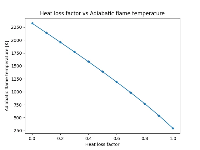
When H_loss_factor is 0, the adiabatic flame temperature is same as the process without any heat loss. With increase in H_loss_factor, the heat of combusiton is lost out of the system and hence the adiabatic flame temperature drops significantly. When heat loss `dQ=dQ_(max)`, the adiabatic flame temperature is approximately equal to initial temperature meaning all the heat of combustion is lost to atmosphere.

3. Adiabatic flame temperature variation with respect to Alkane, Alkene, Alkyne :

Adiabatic flame temperature is to calculated for compunds with 2 carbon atoms in the form of alkane, alkene and alkyne.

The respective stoichiometric combustion of these compounds are as shown below:

Ethane: `C_2H_6 + 3.5(O_2 + 3.76N_2) -> 2CO_2 + 3H_2O + 13.16N_2`

Ethene: `C_2H_4 + 3(O_2 + 3.76N_2) -> 2CO_2 + 2H_2O + 11.28N_2`

Ethyne: `C_2H_2 + 2.5(O_2 + 3.76N_2) -> 2CO_2 + H_2O + 9.4N_2`

In general combusion of hydrocarbon can be estimated using the generic formula

`C_xH_y + (x+y/4)(O_2 + 3.76N_2) -> xCO_2 + (y/2)H_2O + (x+y/4)*3.76N_2`

Adiabatic flame temperature is deduced using Newton-Raphson method as before assuming constant pressure process where total enthalpy remains constant. By solving the following equation with enthalpy represented as a function of temperature, `T_(ad)` is calculated in iterative process

`DeltaH = H_("reactants") - H_("products") = 0`

The python program written to solve the above equation for the 3 organic compunds mentioned above is shown below

"""
Calculation of adabatic flame temperature for combustion of alkane, alkene and alkyne
in constant pressure using NASA's thermodynamic data
alkane: C2H6; alkene: C2H4; alkyne: C2H2
"""
import matplotlib.pyplot as plt

# Constants and inputs
R = 8.314				# Universal gas constant
Ti = 298.15				# Initial temperature
T_init = 1500			# Initial guess value for adiabatic flame temperature
tol = 1e-3				# Tolerance for convergence of T_adiabatic
alpha = 0.8				# Under-relaxation factor
T_ad = []				# Result array - python
counter_arr = []		# iteration counter array
compounds = ["alkane","alkene","alkyne"]

# NASA thermodynamic data
# reactants
c2h6_coeff_l = [4.29142492E+00,-5.50154270E-03, 5.99438288E-05, -7.08466285E-08, 2.68685771E-11, -1.15222055E+04, 2.66682316E+00]
c2h4_coeff_l = [3.95920148E+00, -7.57052247E-03, 5.70990292E-05, -6.91588753E-08, 2.69884373E-11, 5.08977593E+03, 4.09733096E+00]
c2h2_coeff_l = [8.08681094E-01, 2.33615629E-02, -3.55171815E-05, 2.80152437E-08, -8.50072974E-12, 2.64289807E+04, 1.39397051E+01]
o2_coeff_l = [3.78245636E+00, -2.99673416E-03, 9.84730201E-06, -9.68129509E-09, 3.24372837E-12, -1.06394356E+03, 3.65767573E+00]
n2_coeff_l = [0.03298677E+02, 0.14082404E-02, -0.03963222E-04, 0.05641515E-07, -0.02444854E-10, -0.10208999E+04, 0.03950372E+02]
# products
co2_coeff_h = [3.85746029E+00, 4.41437026E-03, -2.21481404E-06, 5.23490188E-10, -4.72084164E-14, -4.87591660E+04, 2.27163806E+00]
h2o_coeff_h = [3.03399249E+00, 2.17691804E-03, -1.64072518E-07, -9.70419870E-11, 1.68200992E-14, -3.00042971E+04, 4.96677010E+00]
n2_coeff_h = [0.02926640E+02, 0.14879768E-02, -0.05684760E-05, 0.10097038E-09, -0.06753351E-13, -0.09227977E+04, 0.05980528E+02]

# calculate heat of formation based on temperature and thermodynamic coeffs
def h(T,coeffs):
	# H = (a1 + a2*T/2 + a3*T^2/3 + a4*T^3/4 + a5*T^4/5 + a6/T) * R * T
	return (coeffs[0] + coeffs[1]*T/2 + coeffs[2]*pow(T,2)/3 + coeffs[3]*pow(T,3)/4 + coeffs[4]*pow(T,4)/5 + coeffs[5]/T) * T * R

# Solve enthalpy balance equation with heat loss and return the residual
def f(T,compound):
	if compound == "alkane":
		# C2H6 + 3.5(O2 + 3.76N2) = 2CO2 + 3H2O + 13.16N2
		h_reactants = h(Ti,c2h6_coeff_l) + 3.5*h(Ti,o2_coeff_l) + 13.16*h(Ti,n2_coeff_l)
		h_products = 2*h(T,co2_coeff_h) + 3*h(T,h2o_coeff_h) + 13.16*h(T,n2_coeff_h)
	elif compound == "alkene":
		# C2H4 + 3(O2 + 3.76N2) = 2CO2 + 2H2O + 11.28N2
		h_reactants = h(Ti,c2h4_coeff_l) + 3*h(Ti,o2_coeff_l) + 11.28*h(Ti,n2_coeff_l)
		h_products = 2*h(T,co2_coeff_h) + 2*h(T,h2o_coeff_h) + 11.28*h(T,n2_coeff_h)
	elif compound == "alkyne":
		# C2H2 + 2.5(O2 + 3.76N2) = 2CO2 + H2O + 9.4N2
		h_reactants = h(Ti,c2h2_coeff_l) + 2.5*h(Ti,o2_coeff_l) + 9.4*h(Ti,n2_coeff_l)
		h_products = 2*h(T,co2_coeff_h) + h(T,h2o_coeff_h) + 9.4*h(T,n2_coeff_h)
	else:
		raise Exception("compound not supported")
	return h_products - h_reactants


# calculate derivative of f(T) using numerical first order Taylor series method
def fprime(T,compound):
	return (f(T+1e-6,compound)-f(T,compound))/1e-6

# Solve for T_adiabatic for given values of H_loss_factor
for compound in compounds:
	T = T_init				# Initialize adiabatic temperature
	counter = 0				# iteration counter
	while abs(f(T,compound)) > tol:
		T = T - alpha * f(T,compound)/fprime(T,compound)
		counter += 1
		if counter > 1000:
			break
	T_ad.append(T)
	counter_arr.append(counter)

plt.bar(compounds,T_ad)
plt.xlabel("compounds")
plt.ylabel("Adiabatic flame temperature [K]")
plt.title("Compounds vs Adiabatic flame temperature")
plt.show()

Result:

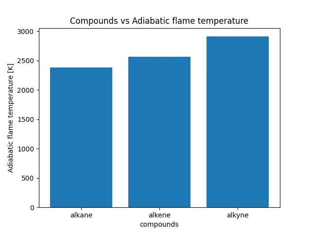
It can be seen that the adiabatic flame temperature increases with decrease in hydrogen atoms in hydrocarbons. Eventhough alkyne and alkene take more energy to break the triple and double carbon-carbon bonds, they produce more heat compared to alkane. More carbon atoms are available per kg in alkene and alkyne compared to alkane due to lesser number of hydrogen atoms. The excess C atoms bond with `O_2`to produce more `CO_2` and hence release much more energy compared to alkanes. With increase in `CO_2` to `H_2O` ratio on products side, the adiabatic flame temperature also increases. Also, per mole of alkyne comsumes less amount of air to combust compared to alkane which reduces the amount of inert heating of products such as `H_2O` and `N_2`.

4. Adiabatic flame temperature variation with respect to number of Carbon atom chains :

Adiabatic flame temperature of alkanes with different number of carbon atoms are to be calculated using Newton-Raphson method as done before with constant pressure assumption. Solving for enthalpy balance equation with enthalpy as a f(T), the adiabatic flame temperature is obtained in iterative process. Using the generic formula for complete combustion of hydrocarbon given below and substituting the values of 1,2 and 3 for x, combusiton of 3 alkane compounds namely methane, ethane and propare are obtained. The generic description of alkane `C_nH_(2n+2)` allows us to deduce y from x using the formula `y = 2x +2`

`C_xH_y + (x+y/4)(O_2 + 3.76N_2) -> xCO_2 + (y/2)H_2O + (x+y/4)*3.76N_2`; x = {1,2,3} and y = 2x + 2

A python program similar to previous one is written to calculate adiabatic flame temperature of different alkane compounds. Switch case statement is used to select the correct NASA coefficients for given number of carbon atoms in alkanes. The generic equation provided is solved with variables x and y instead of separate equations for each compounds. The results are plotted in bar chars. The python program written is as shown below

"""
Calculation of adabatic flame temperature for combustion of alkanes with 
different carbon composition in constant pressure using NASA's thermodynamic data 
methane: CH4; ethane: C2H6; propane: C3H8
"""
import matplotlib.pyplot as plt

# Constants and inputs
R = 8.314				# Universal gas constant
Ti = 298.15				# Initial temperature
T_init = 1500			# Initial guess value for adiabatic flame temperature
tol = 1e-3				# Tolerance for convergence of T_adiabatic
alpha = 0.8				# Under-relaxation factor
T_ad = []				# Result array - python
counter_arr = []		# iteration counter array
c_compositions = range(1,4)	 # carbon composition in alkane


# NASA thermodynamic data
# reactants
ch4_coeff_l = [5.14987613E+00, -1.36709788E-02, 4.91800599E-05, -4.84743026E-08, 1.66693956E-11, -1.02466476E+04, -4.64130376E+00]
c2h6_coeff_l = [4.29142492E+00, -5.50154270E-03, 5.99438288E-05, -7.08466285E-08, 2.68685771E-11,-1.15222055E+04, 2.66682316E+00]
c3h8_coeff_l = [ 0.93355381E+00, 0.26424579E-01, 0.61059727E-05, -0.21977499E-07, 0.95149253E-11, -0.13958520E+05, 0.19201691E+02]
o2_coeff_l = [3.78245636E+00, -2.99673416E-03, 9.84730201E-06, -9.68129509E-09, 3.24372837E-12, -1.06394356E+03, 3.65767573E+00]
n2_coeff_l = [0.03298677E+02, 0.14082404E-02, -0.03963222E-04, 0.05641515E-07, -0.02444854E-10, -0.10208999E+04, 0.03950372E+02]
# products
co2_coeff_h = [3.85746029E+00, 4.41437026E-03, -2.21481404E-06, 5.23490188E-10, -4.72084164E-14, -4.87591660E+04, 2.27163806E+00]
h2o_coeff_h = [3.03399249E+00, 2.17691804E-03, -1.64072518E-07, -9.70419870E-11, 1.68200992E-14, -3.00042971E+04, 4.96677010E+00]
n2_coeff_h = [0.02926640E+02, 0.14879768E-02, -0.05684760E-05, 0.10097038E-09, -0.06753351E-13, -0.09227977E+04, 0.05980528E+02]

# calculate heat of formation based on temperature and thermodynamic coeffs
def h(T,coeffs):
	# H = (a1 + a2*T/2 + a3*T^2/3 + a4*T^3/4 + a5*T^4/5 + a6/T) * R * T
	return (coeffs[0] + coeffs[1]*T/2 + coeffs[2]*pow(T,2)/3 + coeffs[3]*pow(T,3)/4 + coeffs[4]*pow(T,4)/5 + coeffs[5]/T) * T * R

# Solve enthalpy balance equation with heat loss and return the residual
def f(T,c_comp):
	#CxHy + (x+y/4)(O2 + 3.76N2) -> xCO2 + (y/2)H2O + (x+y/4)*3.76N2
	x = c_comp
	y = 2*x + 2
	match c_comp:
		case 1:
			coeff_fuel = ch4_coeff_l
		case 2:
			coeff_fuel = c2h6_coeff_l
		case 3:
			coeff_fuel = c3h8_coeff_l
		case default:
			raise Exception("compund not supported")
	h_reactants = h(Ti,coeff_fuel) + (x + y/4)*h(Ti,o2_coeff_l) + ((x + y/4)*3.76)*h(Ti,n2_coeff_l)
	h_products = x*h(T,co2_coeff_h) + (y/2)*h(T,h2o_coeff_h) + ((x + y/4)*3.76)*h(T,n2_coeff_h)
	return h_products - h_reactants


# calculate derivative of f(T) using numerical first order Taylor series method
def fprime(T,c_comp):
	return (f(T+1e-6,c_comp)-f(T,c_comp))/1e-6

# Solve for T_adiabatic for given values of H_loss_factor
for c_comp in c_compositions:
	T = T_init				# Initialize adiabatic temperature
	counter = 0				# iteration counter
	while abs(f(T,c_comp)) > tol:
		T = T - alpha * f(T,c_comp)/fprime(T,c_comp)
		counter += 1
		if counter > 1000:
			break
	T_ad.append(T)
	counter_arr.append(counter)

plt.bar(c_compositions,T_ad)
plt.xticks(c_compositions)
plt.xlabel("Number of C atoms in alkanes")
plt.ylabel("Adiabatic flame temperature [K]")
plt.title("Alkane Compounds vs Adiabatic flame temperature")
plt.show()

Result:

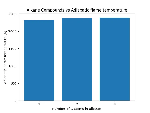
A very mild increase in adiabatic flame temperature is seen with increase in number of carbon atoms in alkane compounds. Eventhough more carbon atoms are present in propare per mole of fuel compared to methane, the raise in adiabatic flame temperature is not significant. This is because, with increase in C atom by x units, H atoms raise by 2x+2 units. Hence the ratio of `CO_2` to `H_2O` on product side increase by a very small margin to increase `T_(ad)` noticeably. Also with increase in C atoms on reactant side, numer of air moles required for complete combustion increases. Hence some of the heat of combustion is used for inert heating of products such as `H_2O` and `N_2`.