Week 7 - Simulation of a 1D Super-sonic nozzle flow simulation using Macormack Method

Isentropic flow through a quasi 1D subsonic-supersonic nozzle:

The nozzle is assumed to be have flow variations in one dimension only - x. Hence the primitive variables such as -> x-velocity(`V`), pressure(`p`), density(`rho`) and temperature(`T`) vary along x but stays constant within the cross-section area at a particular value for x. Cross-section area along the nozzle is assumed to be varying as a function of x. This problem is not truly 1D, but since the area is approximated as a function of x and due to above assumptions, it is considered as quasi 1D problem.Other assumptions made for this problem are: fluid flowing through the nozzle is inviscid, heat generation is zero and body forces are negligible.

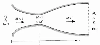
Courtesy: Computational Fluid Dynamics by John D Anderson.

Since, this is a quasi 1D problem and not pure 1D problem, the generic flow equations simplified to 1D cannot be used here. An infinitesimal strip of nozzle length, dx is taken and conservation of mass, momemtum and energy are applied across this strip and integrated to the whole nozzle. Detailed derivation for this 1D quasi flow equations can be found from CFD by John D Anderson.

Non-conservative form of governing equaitons:

Governing equaitons for quasi 1D flow through nozzle are given by the following equations in non-conservative form:

`A(delrho)/(delt) + rhoA(delV)/(delx) + rhoV(delA)/(delx) + VA(delrho)/(delx) = 0` --- (1)

`rho(delV)/(delt) + rhoV(delV)/(delx) = - (delp)/(delx)` --- (2)

`rho(dele)/(delt) + rhoV(dele)/(delx) = -p (delV)/(delx) - pV(del(ln A))/(delx)` --- (3)

Equ (1), (2) and (3) represent continuity, momentum and energy conservation equations respectively.

Using the relation `e = C_vT` for calorifically perfect gas and `C_v = R/(gamma -1)`, equ (3) becomes

`rhoR/(gamma -1)(delT)/(delt) + rhoVR/(gamma -1)(delT)/(delx) = -p (delV)/(delx) - pV(del(ln A))/(delx)` --- (4)

We have 4 unknowns - `p, rho, u and T` and 3 equations. To complete the set of equations, we use the following ideal gas equation

`p = rhoRT` --- (5)

Using equ (1), (2), (4) and (5) primitive variables for flow field in quasi 1D nozzle can be determined.

Non-dimensionalized governing equations:

To follow the convention of using non-dimensionalized variables for the flow field, the primitive variables can be non-dimensionalized as follows:

`T' = T/T_0` `rho' = rho/rho_0` `x' = x/L` `a_0 = sqrt(gammaRT_0)`

`V' = V/a_0` `t' = t/(L//a_0)` `A' = A/(A^**)`

'0' subscript represents properties at the reservoir or inlet. L is the length of the nozzle. `a_0` is the speed of sound at reservoir conditions. `A^**` is throat area of the nozzle.

Substituing equation (5) and it's derivative w.r.t x in equ (2) and (4), variable `p` and it's derivative can be eliminated from the governing equations. Replacing the variables with non-dimensionalized expressions from the above equations for equations (1), (2) and (4) after subsituting for `p` and it's derivatives, we get final forms of non-conservative governing equations in non-dimensional terms.

`(delrho')/(delt) = -rho'(delV')/(delx') - rho'V'(del(ln A'))/(delx') - V'(delrho')/(delx')` ----- (6)

`(delV')/(delt') = -V'(delV')/(delx') - 1/gamma((delT')/(delx')+(T')/(rho')(delrho')/(delx'))` ----- (7)

`(delT')/(delt') = -V'(delT')/(delx') - (gamma -1)T'((delV')/(delx')+V'(del(ln A'))/(delx'))` ----- (8)

Non-dimensionalized pressure is represented as `p' = p/p_0`. Non-dimensionalizing equ (5), we get

`p' = rho'T'` ---- (9)

Equ (9) can be used to obtain the non-dimensionalized pressure if required.

Initial conditions:

A good set of initial guess will allow for the solver to attain steady state much faster. Initial conditions as prescribed in the problem are

`rho' = 1 - 0.3146x` ; `T' = 1-0.2314x` ; `V' = (0.1+1.09x)T^0.5`

Area as a function of x as prescribed in the probelm are

`A' = 1 + 2.2(x-1.5)^2 ;" " 0<=x<=3`

Time step calculation:

Explicit conditions for stability is CFL no, `C` to be less than or equal to 1. From the definition of `C`, `Deltat` can be obtained.

`Deltat = C (Deltax)/(a + V)`

By setting `C=1` and using the values of `Deltax, a and V` at each node corresponding `Deltat` can be obtained for each node. For the solution to have all the nodes at same physical time and a meaningful transient profile, `Deltat` will be used as a constant value for each time-step. This value is calculated by taking the minimum of `Deltat` calculated for all the nodes. For each time-step, `Deltat` is calculated using this method to keep the courant number constant and adapt the time-step size for faster convergence.

Solving the governing equations using MacCormack's method:

To obtain a steady steady solution for the quasi 1D nozzle problem, an initial state is assumed for the varirables inside the nozzle at time, t=0. Boundary conditions in terms of variables or it's derivatives are applied across the boundaries to get an unique solution. Then the solution is calculated for next time-step with `t^(n+1) = t^n + Deltat` using the MacCormack's 2-step process in explicit manner. MacCormcack 2-step process for calculating variables at next time-step are described as follows

1. Predictor step
   1. Using the values of variables at previous time-step, the derivatives, `((delrho')/(delt))_p^n, ((delV')/(delt'))_p^n and ((delT')/(delt'))_p^n` (Subscript "p" for the derivatives denote they are from predictor step) are calculated using equations (6),(7) and (8). Spacial derivatives in these equations are calculated using first order forward differece scheme as shown below
      `(delphi^n)/(delx) = (phi_(i+1)^n - phi_i^n)/(Deltax)`
      where `phi` -> is a representative variable, can be replaced with required variables
      
   2. Flow variables using the predictor time derivatives are calculated as shown below
      `barphi^(n+1) = phi^n + ((delphi)/(delt))_pDeltat`
      where `phi` -> is a representative variable, can be replaced with `rho',V' and T'`. `barphi` shows it's an intermediate value, not final.
2. Corrector step
   1. In this step, the time-derivatives, `((delrho')/(delt))_c^(n+1), ((delV')/(delt'))_c^(n+1) and ((delT')/(delt'))_c^(n+1)` (Subscript c denotes corrector step) are calculated again using equations (6),(7) and (8),but this time using the values of variables from predictor step -> `barrho, barV and barT`. Spacial derivates are calcualted using the values from predictor step, but first order backward difference scheme is used instead such as shown below
      `(delbarphi^(n+1))/(delx) = (barphi_i^(n+1) - barphi_(i-1)^(n+1))/(Deltax)`
      where `barphi` -> is a representative variable, can be replaced with required variables
      
   2. Average time-derivatives, `((delrho')/(delt))_(av), ((delV')/(delt'))_(av) and ((delT')/(delt'))_(av)` are calculated by taking the average of the time-derivatives calculated in predictor and corrector step such as shown below
      `((delphi)/(delt))_(av) = 0.5(((delphi)/(delt))_p^n + ((delbarphi)/(delt))_c^(n+1))`
      where `phi` -> is a representative variable, can be replaced with `rho',V' and T'`.
      
   3. Final values of the flow variables are calculated using the average time-derivatives and variables from previous time-step
      `phi^(n+1) = phi^n + ((delphi)/(delt))_(av)Deltat`
      where `phi` -> is a representative variable, can be replaced with `rho',V' and T'`.
      

This process is done for all the interior nodes in the domain and boundary conditions are applied to the exterior nodes. Multiple time-steps are calculated in this manner until steady state solution is obtained.

Boudary conditions:

Inlet: Since the flow is subsonic at inlet, one characteristic line moves right into the domain and another moves out of the domain. Also the streamline points into the domain. Hence, 2 variables need to be fixed and 1 variable needs to float with the solution. Variables `rho' and T'` can be fixed to a value of 1, which would represents the reservoir condition. Fixing the value of velocity to reservoir condition would mean 0 velocity and hence 0 mass-flow rate. This would not be acceptable as reservoir is assumed be of infinite area, but inlet here has a finite volume. Also the mass-flow rate has to be positive and constant across the nozzle when steady state reaches. Hence the velocity at inlet is calculated using extrapolation from neighboring nodes.

`rho'=1, T'=1 and V_1' = 2V_2'-V_3'`

Outlet: Since the flow at outlet is supersonic, both the characteristic lines move out of the domain and streamline also points out of the domain. Hence all 3 variables are allowed to float with time. In other words, supersonic flow doesn't affect upstream conditions. Hence, all 3 variables are extrapolated from neighboring nodes.

`phi_N' = 2phi_(N-1)' - phi_(N-2)'` where `phi` -> is a representative variable, can be replaced with `rho',V' and T'`.

These boundary conditions are applied at each time-step after the calculation of solution variables at interior nodes.

Matlab Program:

A matlab function is written to solve the quasi 1D nozzle flow equations using non-conservative method. The funtion takes the domain information, initial conditions of primitive variables, number of time-steps and constants such as courant number and gamma as inputs. After solving the equations, the function returns the final distribution of primitive variables, history of primitive variables at throat during the solution and mass-flow rate distribution at a few prescribed time-steps.

function [rho,v,t,rho_hist,v_hist,t_hist,mf_hist] ...
    = non_conservative(x,a,rho,v,t,nt,C,gamma)
% Non-conservative form of quasi 1D nozzle flow governing equation:

% number of grid points
np = length(x);
% length of nozzle
L = x(end);
% distance between grid points
dx = L / (np - 1);    

% mass-flow-history counter
mf_hist_no = 1;
mf_hist_array = [50 100 200 400 800 1400];

% Loop for time marching
for i = 1:nt

    %backup of previous time-step flow-variables
    rho_old = rho;
    v_old = v;
    t_old = t;

    % time-step calculation
    a_s = sqrt(t);             % non-dimensionalized speed of sound
    dt = C * dx/max(a_s + v);
    
    %predictor step - loop over inner nodes
    for j = 2:np-1

        % calculate space derivatives using 1st order forward differencing
        dv_dx = (v(j+1) - v(j))/dx;
        dloga_dx = (log(a(j+1)) - log(a(j)))/dx;
        drho_dx = (rho(j+1) - rho(j))/dx;
        dt_dx = (t(j+1) - t(j))/dx;

        % continuity equ
        drho_dt_p(j) = - rho(j)*dv_dx - rho(j)*v(j)*dloga_dx - v(j)*drho_dx;
        %momentum equ
        dv_dt_p(j) = - v(j)*dv_dx - (1/gamma)*(dt_dx + (t(j)/rho(j))*drho_dx);
        %energy equ
        dt_dt_p(j) = -v(j)*dt_dx - (gamma - 1)*t(j)*(dv_dx + v(j)*dloga_dx);

        % calculate flow variables
        rho(j) = rho(j) + drho_dt_p(j)*dt;
        v(j) = v(j) + dv_dt_p(j)*dt;
        t(j) = t(j) + dt_dt_p(j)*dt;
    end

    % corrector step
    % loop over inner nodes
    for k = 2:np-1
        
        % calculate space derivatives using 1st order backward differencing
        dv_dx = (v(k) - v(k-1))/dx;
        dloga_dx = (log(a(k)) - log(a(k-1)))/dx;
        drho_dx = (rho(k) - rho(k-1))/dx;
        dt_dx = (t(k) - t(k-1))/dx;

        % continuity equ
        drho_dt_c(k) = - rho(k)*dv_dx - rho(k)*v(k)*dloga_dx - v(k)*drho_dx;
        %momentum equ
        dv_dt_c(k) = - v(k)*dv_dx - (1/gamma)*(dt_dx + (t(k)/rho(k))*drho_dx);
        %energy equ
        dt_dt_c(k) = -v(k)*dt_dx - (gamma - 1)*t(k)*(dv_dx + v(k)*dloga_dx);
    end

    % calcuate average time-derivatives
    drho_dt_av = 0.5*(drho_dt_p + drho_dt_c);
    dv_dt_av = 0.5*(dv_dt_p + dv_dt_c);
    dt_dt_av = 0.5*(dt_dt_p + dt_dt_c);

    % calculate flow variables
    for l = 2:np-1
        rho(l) = rho_old(l) + drho_dt_av(l)*dt;
        v(l) = v_old(l) + dv_dt_av(l)*dt;
        t(l) = t_old(l) + dt_dt_av(l)*dt;
    end

    % Boundary conditions
    %inlet
    v(1) = 2*v(2) - v(3);
    %outlet
    rho(np) = 2*rho(np-1) - rho(np-2);
    v(np) = 2*v(np-1) - v(np-2);
    t(np) = 2*t(np-1) - t(np-2);

    % Solution monitor
    rho_hist(i) = rho((np+1)/2);
    v_hist(i) = v((np+1)/2);
    t_hist(i) = t((np+1)/2);

    % save mass-flow development every 250 time-steps
    if ismember(i, mf_hist_array)
        mf_hist(mf_hist_no,:) = (rho .* a .* v)';
        mf_hist_no = mf_hist_no + 1;
    end
end

end

Conservative form of governing equations:

`del/(delt)(rhoA) + del/(delx)(rhoAV) = 0` --- (10)

`del/(delt)(rhoAV) + del/(delx)(rhoAV^2) = - A (dp)/(dx)` ---- (11)

`del/(delt)(rho(e+V^2/2)A) + del/(delx)(rho(e+V^2/2)VA) = - (del(pAV))/(delx)` ---(12)

The set of governing equations provided above represent continuity, momentum and energy conservation equations for a quasi 1D flow. These are derived by applying the conservating principles to an infinitesimal strip of a converging-diverging nozzle and integrating it to the whole nozzle. Detailed derivation is available in CFD by John.D Anderson.

Non-dimensionalized conservative governing equations:

Same set of non-dimensionalizing equation used for non-conservative form is used here to repace the flow varables in above equations with non-dimensionalized varaibles. Energy term `e` is non-dimensionalized as `e' = e/e_0`. After applying these non-dimensional transformations the final governing equation in non-dimensional consevative form is as shown below

`(del(rho'A'))/(delt') + (del(rho'A'V'))/(delx') = 0` --- (13)

`(del(rho'A'V'))/(delt') + (del(rho'A'V'^2 + (1//gamma)p'A'))/(delx') = 1/gammap'(delA')/(delx')` ----(14)

`(del(rho'((e')/(gamma -1)+gamma/2V'^2)A'))/(dt')+(del(rho'((e')/(gamma-1)+gamma/2V'^2)V'A'+p'A'V'))/(delx') = 0` ---- (15)

Using the calorifically perfect gas relation for e,

`e' = (C_vT)/(C_vT_0) = T'`

Hence, `e'` can be replaced with `T'` in equ (15)

These equations, can be represented in a generic format such as

`(delU)/(delt') = - (delF)/(delx') + J` --- (16)

where U, F and J are 3-dimensional vectors namely -- solution vector, Flux vector and source term vector respectively. The elements of these vectors that satify the equ (13), (14) and (15) are as given below

`U_1 = rho'A'`; `F_1 = rho'A'V'`; `J_1 = 0`

`U_2 = rho'A'V'`; `F_2 = rho'A'V'^2 + 1/gammap'A'`; `J_2 = 1/gammap'(delA')/(delx')`

`U_3 = rho'((T')/(gamma-1)+gamma/2V'^2)A'`; `F_3 = rho'((T')/(gamma-1)+gamma/2V'^2)V'A'+p'A'V'`; `J_3 = 0`

Since, we have 4 unknowns - `rho,V,T and p` and only 3 equation, we can use ideal gas equation, equ (9) to complete the problem.

The solution vectors can be calculated using the MacCormack method as described above using the values of flux and source vectors from previous time-step. Primitive variables can then be calculated using the following expressions derived from the description of these vectors above and equ (9).

`rho' = U_1/(A')` ; `V' = U_2/U_1` ; `T' = (gamma-1)(U_3/U_1 - gamma/2V'^2)` ; `p' = rho'T'`

Conservative equation in pure form:

But in this method, primitive varaibles have to be calculated for each time-step from the `U` vector and then used to calculate `F` and `J` vectors for next time-step. Due this complexity, the solution may become unstable occasionally and hence a pure form of solution is preferred where the vectors - `F` and `J` are calculated purely based on `U` vector without the need to use primitive variables. This can be done using the expressions to define the vector elements using primitive variables and the expressions to define primitive varirables from the vector elements. Variable `p'` is eliminated from the vector element expressions using equ (9) and other variables are substitued with expressions involving `U` elements.

`F_1 = U_2`; `J_1 = 0`

`F_2 = U_2^2/U_1 + (gamma-1)/gamma(U_3-gamma/2U_2^2/U_1)`; `J_2 = (gamma-1)/gamma(U3-gamma/2U_2^2/U_1)(del(ln A'))/(delx')`

`F_3 = gamma(U_2U_3)/U_1 - (gamma(gamma-1))/2U_2^3/U_1^2`; `J_3 = 0`

Using the above expressions, equ (16) can be directly solve for U with F and J as functions of U.

Initial Conditions:

As prescribed, the boundary conditions are

`rho' = 1, T'=1 ; " for " 0<=x'<=0.5`

`rho' = 1-0.366(x'-0.5), T'=1-0.167(x'-0.5) ; " for " 0.5<=x'<=1.5`

`rho' = 0.634-0.3879(x'-1.5), T'=0.833-0.3507(x'-1.5) ; " for " 1.5<=x'<=3.5`

`V'=U_2/(rho'A')` --> from the definition of `U_2`. `U_2`(mass-flow-rate) is assumed to be 0.59 for initial step.

Area is defined as a function of `x` which is the same used for non-conservative method

`A' = 1 + 2.2(x-1.5)^2 ;" " 0<=x<=3`

Time-step calculation:

Same approach defined for non-conservative method is used to determine the time-step size for each time-step.

`Deltat = C (Deltax)/(a + V)` , with `C = 1`

Solving the governing equations using MacCormack method:

The approach is same as defined for non-conservative method, only this time, we'd need to use the vector elements of U,F and J instead of primitive variables for the solution process.

1. Flux and source vector elements are calculated based on initial conditions for all nodes
2. Predictor step
   1. Space derivatives of flux elements are calculated based on first order forward differencing
   2. Time-derivatives of solution elements are calculated using the governing equations based on previous time-step flux variable values
   3. Current values of solution elements are calculated using the time-derivative obtained
3. Corrector step
   1. Re-calculate the flux vector elements based on predictor step solution vector element values
   2. Calculate space derivatives of flux elements using first order backward differecing scheme
   3. Calculate the time-derivatives of solution vector elements using updated values of flux elements
   4. Obtain the average of time-derivatives calculated in predictor and corrector step
   5. Calculate final values of soltuion vector elememts based on the average time-derivatives.
4. Calculate the primitive variables from solution vector results and calculate the time-step size for next time-step
5. Repeat from step 2 until steady-state solution is obtained

Boundary conditions:

Boundary conditions remain the same as for the non-conservative form since the underlying problem is the same. But, they need to be applied in terms of U,F and J vector elements since we are dealing with pure form of conservative solution. Hence the same boundary conditions described for non-conservative form needs to be expressed in terms of U,F and J vector using definition of these vector elements.

Let `i` represent the node index,

Inlet:

`U_(1(i=1)) = (rho'A')_(i=1) = A'_(i=1) , "since " rho'_(i=1) = 1`

`U_(2(i=1)) =2U_(2(i=2))-U_(2(i=3))` --> allowed to float

`U_(3(i=1)) = (rho'A'((T')/(gamma-1) -gamma/2V'^2))_(i=1) = U_(1(i=1))(1/(gamma-1) + gamma/2V'_(i=1)^2), "since " T'_(i=1)=1`

Outlet: (all the solution vector elements are allowed to float)

`U_(1(i=N))=2U_(1(i=N-1)) - U_(1(i=N-2))`, where "N" represents number of grid points

`U_(2(i=N))=2U_(2(i=N-1)) - U_(2(i=N-2)`

`U_(3(i=N))=2U_(3(i=N-1)) - U_(3(i=N-2)`

These boundary conditions are applied at each time-step after the calculation of solution variables at interior nodes.

Matlab Program:

The conservative form of matlab function also takes inputs similar to those as non-conservative form. It then converts the primitive variables to dependent variables and solves them using the conservative governing equations. Primitive variables are again derived from dependent variables and returned as output of the function. Along with the final variables, the history of primitive variables at throat and mass flow rate distribution at few prescribed time-steps are also returned as outputs.

function [rho,v,t,rho_hist,v_hist,t_hist,mf_hist] ...
    = conservative(x,a,rho,v,t,nt,C,gamma)
% Conservative form of quasi 1D nozzle flow governing equation:

% number of grid points
np = length(x);
% length of nozzle
L = x(end);
% distance between grid points
dx = L / (np - 1);  

% Solution vector
U1 = rho .* a;
U2 = rho .* a .* v;
coeff7 = gamma - 1;
coeff8 = gamma/2;
U3 = rho .* ((t./coeff7) + (coeff8 * v.^2)) .* a;

% mass-flow-history counter
mf_hist_no = 1;
mf_hist_array = [50 100 200 400 800 1400];

% Loop for time marching
for i = 1:nt

    %backup of previous time-step solution vectors
    U1_old = U1;
    U2_old = U2;
    U3_old = U3;

    %Calculate dependent variables
    [F1,F2,F3] = calc_dependent_vars(U1,U2,U3,gamma);
   
    % time-step calculation
    a_s = sqrt(t);
    dt = min(C * (dx./(a_s + v)));
    
    %predictor step - loop over inner nodes
    for j = 2:np-1

        % calculate J2
        da_dx = (a(j+1) - a(j))/dx;
        J2 = (1/gamma) * rho(j) .* t(j) .* da_dx;

        % calculate space derivatives using 1st order forward differencing
        dF1_dx = (F1(j+1) - F1(j))/dx;
        dF2_dx = (F2(j+1) - F2(j))/dx;
        dF3_dx = (F3(j+1) - F3(j))/dx;

        % continuity equ
        dU1_dt_p(j) = - dF1_dx;
        %momentum equ
        dU2_dt_p(j) = - dF2_dx + J2; 
        %energy equ
        dU3_dt_p(j) = - dF3_dx;

        % calculate solution vector - intermediate values
        U1(j) = U1(j) + dU1_dt_p(j)*dt;
        U2(j) = U2(j) + dU2_dt_p(j)*dt;
        U3(j) = U3(j) + dU3_dt_p(j)*dt;
    end

    % Calculate primitve variables
    rho = U1 ./ a;
    v = U2 ./ U1;
    coeff5 = gamma - 1;
    coeff6 = gamma/2;
    U3_by_U1 = U3 ./ U1;
    t = coeff5 * (U3_by_U1 - (coeff6 * v.^2));

    % Boundary conditions
    %inlet
    U2(1) = 2*U2(2) - U2(3);
    v(1) = U2(1) ./ U1(1);
    coeff3 = 1/(gamma - 1);
    coeff4 = gamma/2;
    U3(1) = U1(1) * (coeff3 + (coeff4 * v(1)^2));
    %outlet
    U1(np) = 2*U1(np-1)  - U1(np-2);
    U2(np) = 2*U2(np-1)  - U2(np-2);
    U3(np) = 2*U3(np-1)  - U3(np-2);

    %Calculate dependent variables - intermediate values
    [F1,F2,F3] = calc_dependent_vars(U1,U2,U3,gamma);

    % corrector step
    % loop over inner nodes
    for k = 2:np-1

        % calculate J2
        da_dx = (a(k) - a(k-1))/dx;
        J2 = (1/gamma) * rho(k) .* t(k) .* da_dx;
        
        % calculate space derivatives using 1st order backward differencing
        dF1_dx = (F1(k) - F1(k-1))/dx;
        dF2_dx = (F2(k) - F2(k-1))/dx;
        dF3_dx = (F3(k) - F3(k-1))/dx;

        % continuity equ
        dU1_dt_c(k) = - dF1_dx;
        %momentum equ
        dU2_dt_c(k) = - dF2_dx + J2; 
        %energy equ
        dU3_dt_c(k) = - dF3_dx;
    end

    % calcuate average time-derivatives
    dU1_dt_av = 0.5*(dU1_dt_p + dU1_dt_c);
    dU2_dt_av = 0.5*(dU2_dt_p + dU2_dt_c);
    dU3_dt_av = 0.5*(dU3_dt_p + dU3_dt_c);

    % calculate solution variables
    for l = 2:np-1
        U1(l) = U1_old(l) + dU1_dt_av(l)*dt;
        U2(l) = U2_old(l) + dU2_dt_av(l)*dt;
        U3(l) = U3_old(l) + dU3_dt_av(l)*dt;
    end

    % Boundary conditions
    %inlet
    U2(1) = 2*U2(2) - U2(3);
    v(1) = U2(1) ./ U1(1);
    coeff3 = 1/(gamma - 1);
    coeff4 = gamma/2;
    U3(1) = U1(1) * (coeff3 + (coeff4 * v(1)^2));
    %outlet
    U1(np) = 2*U1(np-1)  - U1(np-2);
    U2(np) = 2*U2(np-1)  - U2(np-2);
    U3(np) = 2*U3(np-1)  - U3(np-2);

    % Calculate primitve variables
    rho = U1 ./ a;
    v = U2 ./ U1;
    coeff5 = gamma - 1;
    coeff6 = gamma/2;
    U3_by_U1 = U3 ./ U1;
    t = coeff5 * (U3_by_U1 - (coeff6 * v.^2));

    % Solution monitor
    rho_hist(i) = rho((np+1)/2);
    v_hist(i) = v((np+1)/2);
    t_hist(i) = t((np+1)/2);

    % save mass-flow development every 250 time-steps
    if ismember(i, mf_hist_array)
        mf_hist(mf_hist_no,:) = U2';
        mf_hist_no = mf_hist_no + 1;
    end
end


end

For the above function, a helper function is written to calculate flux variables from the solution variables.

function [F1,F2,F3] = calc_dependent_vars(U1,U2,U3,gamma)
% Calculate the flux vectors based on solution vector for quasi
% 1D conservative form of governing equations

F1 = U2;

U2_sq_by_U1 = (U2.^2) ./ U1;
coeff1 = (gamma-1)/gamma;
coeff2 = gamma/2;
F2 = U2_sq_by_U1 + (coeff1 * (U3 - (coeff2 * U2_sq_by_U1)));

U2_cube_by_U1_sq = (U2.^3) ./ (U1.^2);
U2_U3_by_U1 = (U2 .* U3) ./ U1;
coeff3 = (gamma * (gamma - 1))/2;
F3 = (gamma * U2_U3_by_U1) - (coeff3 * U2_cube_by_U1_sq);

end

Main program:

The main program defines the domain, constants and initial conditions. It calls non-conservative or conservative forms of solution to solve the problem based on the value of "method" variable defined. Post-processing is done using the return values from the solve functions.

% Solve quasi 1D nozzle flow using MacCormack method
clear all
close all
clc

% Define domain
L = 3;                  % non-dimensional length of domain.
np = 31;                % number of grid points
x = linspace(0,L,np);   % array that hold the the grid points
a = 1 + (2.2*((x-1.5).^2)); % Area as a function of x

% time step parameters
nt = 1400;              % max number of time-steps
C = 0.5;                % courant number  

% Other quantities
gamma = 1.4;            % ratio of specific heats
method = 1;             % 1 for non-conservative and 2 for conservative

% Intial conditions --> non-conservative form
rho_nc = 1 - 0.3146*x;     % non-dimensional density
t_nc = 1 - 0.2314*x;       % non-dimensional temperature 
v_nc = (0.1 + 1.09*x).*t_nc.^0.5; % non-dimensioanl velocity

% Intital Conditons --> conservative form
% non-dimensional density
rho_c = zeros(1,np);
rho_c(x<=0.5) = 1;
rho_c(x>=0.5 & x<=1.5) = 1 - 0.366*(x(x>=0.5 & x<=1.5) - 0.5);
rho_c(x>=1.5 & x<=3.5) = 0.634 - 0.3879*(x(x>=1.5 & x<=3.5) - 1.5);
% non-dimensional temperature
t_c = zeros(1,np);
t_c(x<=0.5) = 1;
t_c(x>=0.5 & x<=1.5) = 1 - 0.167*(x(x>=0.5 & x<=1.5) - 0.5);
t_c(x>=1.5 & x<=3.5) = 0.833 - 0.3507*(x(x>=1.5 & x<=3.5) - 1.5);
% non-dimensioanl velocity
v_c = 0.59 ./ (rho_c .* a);   % assume constant mass-flow rate = 0.59

if method == 1
    % calculate solution in using non-conservation equ
    [rho,v,t,rho_hist,v_hist,t_hist,mf_hist] ...
        = non_conservative(x,a,rho_nc,v_nc,t_nc,nt,C,gamma);
else
    % calculate solution in using conservation equ
    [rho,v,t,rho_hist,v_hist,t_hist,mf_hist] ...
        = conservative(x,a,rho_c,v_c,t_c,nt,C,gamma);
end

% Post_process
% primitive variables distribution
figure(1)
plot(x,t)
hold on
plot(x,v)
plot(x,rho)
xlabel("non-dimensional nozzle length")
ylabel("non-dimensional primitive variables")
title("Non-dimensionalised primitive variable distribution")
legend("temperature","velocity","density")
hold off

% Solution monitor
figure(2)
plot(rho_hist);
hold on
plot(v_hist)
plot(t_hist)
xlabel("time-step")
ylabel("non-dimensional primitive variables")
title("solution monitor at throat")
legend("density","velocity","temperature")

% Mass-flow rate development
figure(3)
mf_hist_array = [50 100 200 400 800 1400];
plot(x,mf_hist)
%legend(time_step(2:end))
xlabel("non-dimensional nozzle length")
ylabel("non-dimensional mass-flow-rate")
legend(string(mf_hist_array))

Results:

Solution is completed using both non-conservative and conservative forms by changing the "method" variable value and following results are obtained.

Non-conservative	Conservative

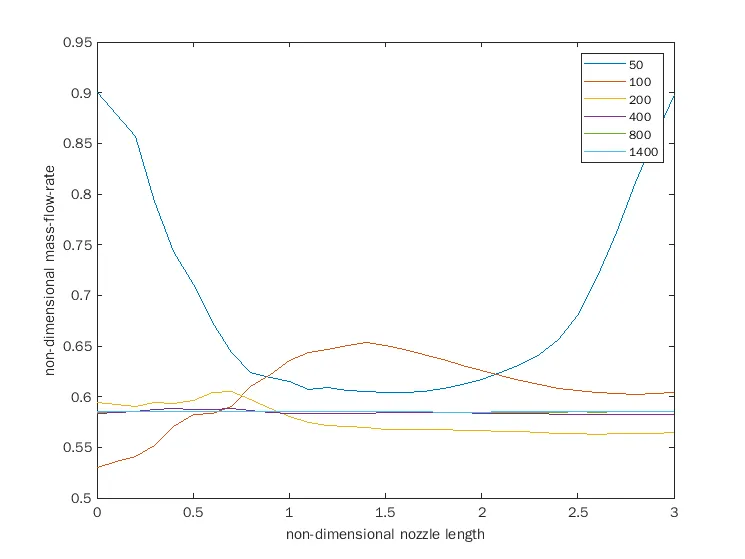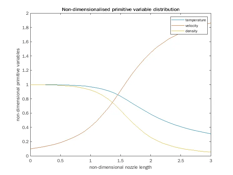
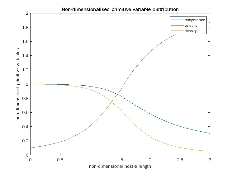
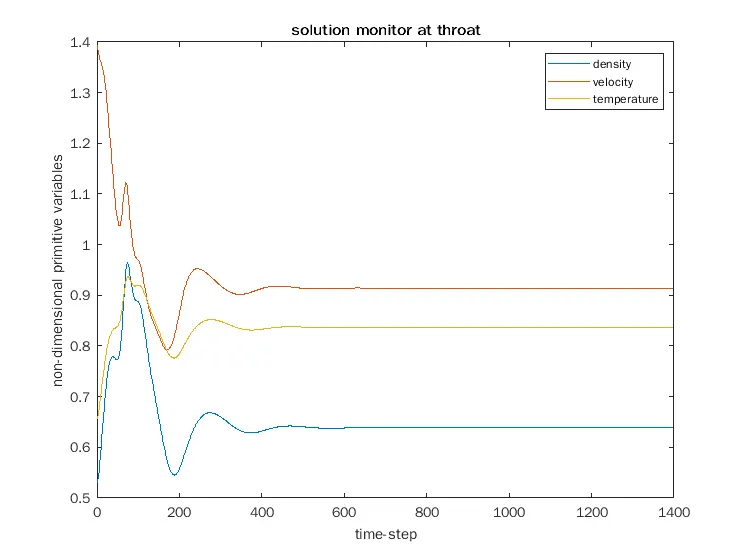
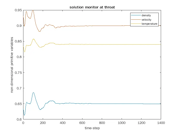
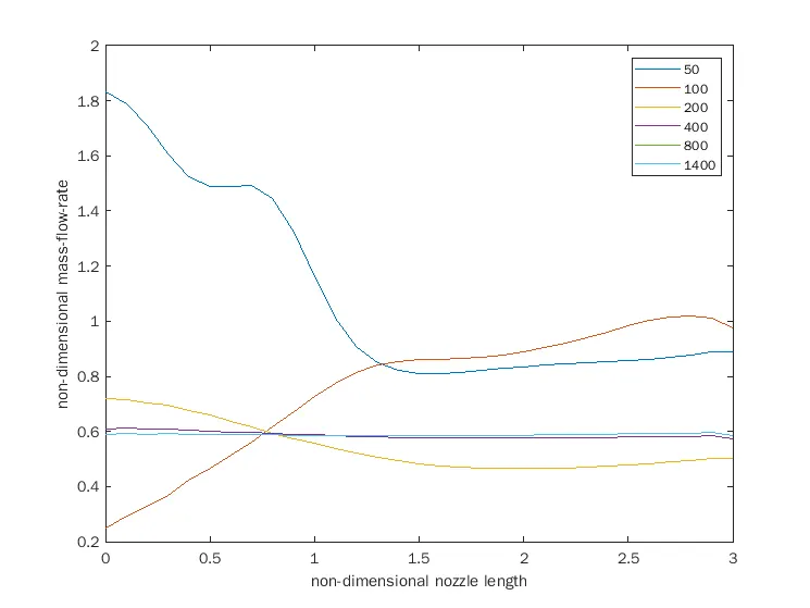
Row 1 shows the comparison of final primitive variable results for the nozzle using non-conservative and conservative methods respectively. There is not much to differentiate between these 2 plots. Solution monitor plots in row2 shows that non-conservative method reaches steady state at around 600 time-steps. Conservative form is provided with better initial conditions where the variable values are close to final values. Even with these set of initial conditions, it takes slightly longer number of time-steps --> around 650, to reach steady state. Final row shows the mass-flow rate development inside the nozzle at different time-steps. After around 400 time-steps, the mass-flow rate seems to have reached a constant value for both the approaches.

Grid independent study:

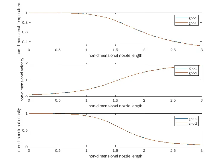
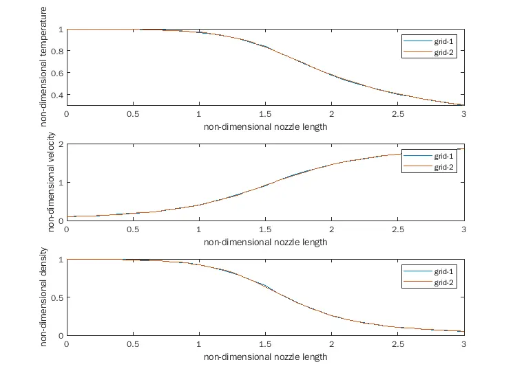
Grid independent study is performed for any CFD based solution approach. Since the derivatives are accurate when `Deltax` tends to 0, there will always be a finite error when calculating CFD solutions with a finite `Deltax` value. The error will subside with reduction in `Deltax`, however with an increased computational cost and it's not-possible to do a numerical approach with 0 `Deltax`. Hence based on the level of accuracy required for the application, the grid size to be used for the solution is decided by conducting a grid independent study. Here we perform a grid independent study using 2 grids as an initial step with second grid twice as dense as the first one.

A matlab program is written to solve the conservative and non-conservative forms of governing equations with 2 grids and compare the results between the grids for each method.

% Perform grid independent study on conservative and non-conservative forms
clear all
close all
clc

% Define domain
L = 3;                  % non-dimensional length of domain.

% time step parameters
nt = 1400;              % max number of time-steps
C = 0.5;                % courant number  

% Other quantities
gamma = 1.4;            % ratio of specific heats
method = 2;             % 1 for non-conservative and 2 for conservative

% Grid independent study
if method == 1
    % grid 1
    np1 = 31;                % number of grid points
    x1 = linspace(0,L,np1);   % array that hold the the grid points
    a1 = 1 + (2.2*((x1-1.5).^2)); % Area as a function of x

    % Intial conditions --> non-conservative form
    rho_nc = 1 - 0.3146*x1;     % non-dimensional density
    t_nc = 1 - 0.2314*x1;       % non-dimensional temperature 
    v_nc = (0.1 + 1.09*x1).*t_nc.^0.5; % non-dimensioanl velocity
    [rho1,v1,t1,rho_hist1,v_hist1,t_hist1,mf_hist1] ...
        = non_conservative(x1,a1,rho_nc,v_nc,t_nc,nt,C,gamma);

    % grid 2
    np2 = 61;                % number of grid points
    x2 = linspace(0,L,np2);   % array that hold the the grid points
    a2 = 1 + (2.2*((x2-1.5).^2)); % Area as a function of x

    % Intial conditions --> non-conservative form
    rho_nc = 1 - 0.3146*x2;     % non-dimensional density
    t_nc = 1 - 0.2314*x2;       % non-dimensional temperature 
    v_nc = (0.1 + 1.09*x2).*t_nc.^0.5; % non-dimensioanl velocity
    [rho2,v2,t2,rho_hist2,v_hist2,t_hist2,mf_hist2] ...
        = non_conservative(x2,a2,rho_nc,v_nc,t_nc,nt,C,gamma);
else 
    % grid 1
    np1 = 31;                % number of grid points
    x1 = linspace(0,L,np1);   % array that hold the the grid points
    a1 = 1 + (2.2*((x1-1.5).^2)); % Area as a function of x

    % Intital Conditons --> conservative form
    % non-dimensional density
    rho_c = zeros(1,np1);
    rho_c(x1<=0.5) = 1;
    rho_c(x1>=0.5 & x1<=1.5) = 1 - 0.366*(x1(x1>=0.5 & x1<=1.5) - 0.5);
    rho_c(x1>=1.5 & x1<=3.5) = 0.634 - 0.3879*(x1(x1>=1.5 & x1<=3.5) - 1.5);
    % non-dimensional temperature
    t_c = zeros(1,np1);
    t_c(x1<=0.5) = 1;
    t_c(x1>=0.5 & x1<=1.5) = 1 - 0.167*(x1(x1>=0.5 & x1<=1.5) - 0.5);
    t_c(x1>=1.5 & x1<=3.5) = 0.833 - 0.3507*(x1(x1>=1.5 & x1<=3.5) - 1.5);
    % non-dimensioanl velocity
    v_c = 0.59 ./ (rho_c .* a1);   % assume constant mass-flow rate = 0.59

    [rho1,v1,t1,rho_hist1,v_hist1,t_hist1,mf_hist1] ...
        = conservative(x1,a1,rho_c,v_c,t_c,nt,C,gamma);
    % grid 2
    np2 = 61;                % number of grid points
    x2 = linspace(0,L,np2);   % array that hold the the grid points
    a2 = 1 + (2.2*((x2-1.5).^2)); % Area as a function of x

    % Intital Conditons --> conservative form
    % non-dimensional density
    rho_c = zeros(1,np2);
    rho_c(x2<=0.5) = 1;
    rho_c(x2>=0.5 & x2<=1.5) = 1 - 0.366*(x2(x2>=0.5 & x2<=1.5) - 0.5);
    rho_c(x2>=1.5 & x2<=3.5) = 0.634 - 0.3879*(x2(x2>=1.5 & x2<=3.5) - 1.5);
    % non-dimensional temperature
    t_c = zeros(1,np2);
    t_c(x2<=0.5) = 1;
    t_c(x2>=0.5 & x2<=1.5) = 1 - 0.167*(x2(x2>=0.5 & x2<=1.5) - 0.5);
    t_c(x2>=1.5 & x2<=3.5) = 0.833 - 0.3507*(x2(x2>=1.5 & x2<=3.5) - 1.5);
    % non-dimensioanl velocity
    v_c = 0.59 ./ (rho_c .* a2);   % assume constant mass-flow rate = 0.59

    [rho2,v2,t2,rho_hist2,v_hist2,t_hist2,mf_hist2] ...
        = conservative(x2,a2,rho_c,v_c,t_c,nt,C,gamma);
end


% % primitive variables distribution
subplot(3,1,1)
plot(x1,t1)
hold on
plot(x2,t2)
xlabel("non-dimensional nozzle length")
ylabel("non-dimensional temperature")
legend("grid-1","grid-2")

subplot(3,1,2)
plot(x1,v1)
hold on
plot(x2,v2)
xlabel("non-dimensional nozzle length")
ylabel("non-dimensional velocity")
legend("grid-1","grid-2")

subplot(3,1,3)
plot(x1,rho1)
hold on
plot (x2,rho2)
xlabel("non-dimensional nozzle length")
ylabel("non-dimensional density")
legend("grid-1","grid-2")

error_t = abs(t1((np1+1)/2) - t2((np1+1)/2)) / abs(t1((np1+1)/2));
error_v = abs(v1((np1+1)/2) - v2((np1+1)/2)) / abs(v1((np1+1)/2));
error_rho = abs(rho1((np1+1)/2) - rho2((np1+1)/2)) / abs(rho1((np1+1)/2));
fprintf("error percentage at throat \n temperature: %f\n velcity: %f\n density: %f",...
    error_t, error_v, error_rho);

Results:

The results from grid independent study is as shown below

Non-conservative	Conservative

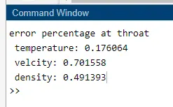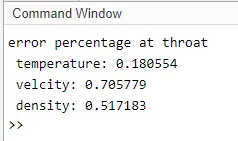
First row shows the final primitive variable profiles for grid1 and grid2 using non-conservative and conservative methods. As can be seen the profiles do overlap and not any noticible difference is seen for both the schemes. Second row shows the error percentage between the grids for primitive variables at nozzle throat. Here as well, the max difference observated is 0.7% which is negligible for our purpose of this study. Hence, the results with original grid with 31 number of points satisfies as grid independent solution.

Comparison of mass-flow rate profiles between non-conservative and conservative forms:

A new matlab program is written is make use of the old non-conservative and conservative functions and obtain the mass-flow distribution along the nozzle after the solution is complete.

% Compare mass-flow distribution between non-conservative 
% and conservative forms
clear all
close all
clc

% Define domain
L = 3;                  % non-dimensional length of domain.
np = 31;                % number of grid points
x = linspace(0,L,np);   % array that hold the the grid points
a = 1 + (2.2*((x-1.5).^2)); % Area as a function of x

% time step parameters
nt = 1400;              % max number of time-steps
C = 0.5;                % courant number  

% Other quantities
gamma = 1.4;            % ratio of specific heats
method = 1;             % 1 for non-conservative and 2 for conservative

% Intial conditions --> non-conservative form
rho_nc = 1 - 0.3146*x;     % non-dimensional density
t_nc = 1 - 0.2314*x;       % non-dimensional temperature 
v_nc = (0.1 + 1.09*x).*t_nc.^0.5; % non-dimensioanl velocity

% Intital Conditons --> conservative form
% non-dimensional density
rho_c = zeros(1,np);
rho_c(x<=0.5) = 1;
rho_c(x>=0.5 & x<=1.5) = 1 - 0.366*(x(x>=0.5 & x<=1.5) - 0.5);
rho_c(x>=1.5 & x<=3.5) = 0.634 - 0.3879*(x(x>=1.5 & x<=3.5) - 1.5);
% non-dimensional temperature
t_c = zeros(1,np);
t_c(x<=0.5) = 1;
t_c(x>=0.5 & x<=1.5) = 1 - 0.167*(x(x>=0.5 & x<=1.5) - 0.5);
t_c(x>=1.5 & x<=3.5) = 0.833 - 0.3507*(x(x>=1.5 & x<=3.5) - 1.5);
% non-dimensioanl velocity
v_c = 0.59 ./ (rho_c .* a);   % assume constant mass-flow rate = 0.59

% calculate solution in using non-conservation equ
[~,~,~,~,~,~,mf_hist1] ...
    = non_conservative(x,a,rho_nc,v_nc,t_nc,nt,C,gamma);
% calculate solution in using conservation equ
[~,~,~,~,~,~,mf_hist2] ...
    = conservative(x,a,rho_c,v_c,t_c,nt,C,gamma);


% Post_process
% Mass-flow rate final
plot(x,mf_hist1(end,:))
hold on
plot(x,mf_hist2(end,:))
xlabel("non-dimensional nozzle length")
ylabel("non-dimensional mass-flow-rate")
legend("non conservative","conservative")

Results:

The final mass-flow rate distribution is plotted against nozzle length for both the solution processes.

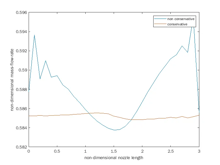
Note that the scale on the y-axis is much smaller. Even though the profiles looks as a non-constant line, with the level of accuracy required, mass-flow rate can still be considered as constant along the nozzle. That said, conservative form of governing equations tend to follow the constant line profile much better compared to non-conservative form. This could be due the fact that conservative form solves for dependent solution varaibles, one of which -> U2 reprensents mass-flow rate. Hence, conservative form of governing equation provides better mass conservation. Although conservative form of governing equations takes a little longer to reach steay-state and more coding effort.