Week 8 - Simulation of a backward facing step in OpenFOAM
Transient Incompressible-laminar-viscous flow simulation through a backward facing step:
1. Uniform Mesh:
IcoFoam solver is used to solve transient incompressible laminar flow problems in openFoam. Hence the same is chosen for our simulaiton here. Couple of tutorials are available for icoFoam solver in the package -> cavity and elbow. Since, neither of these represent our geometry, we could start from any one of them and modify the geometry for our purpose. Here cavity tutorial is copied to $FOAM_RUN folder and renamed to suitably such as backward_step. There are multiple cavity simulation folders inside cavity tutorial. For our purpose we remove everything except cavity.
1a. Meshing
"blockMeshDict" file inside systems folder is edited to represent our problem as suggested in following figures.
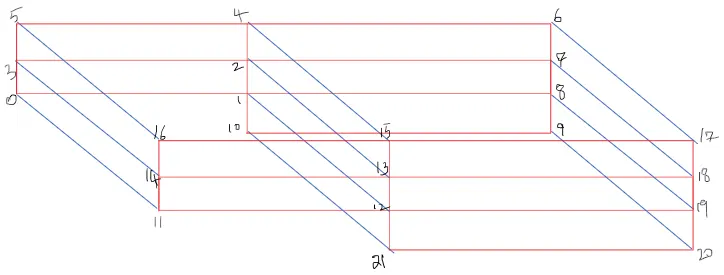
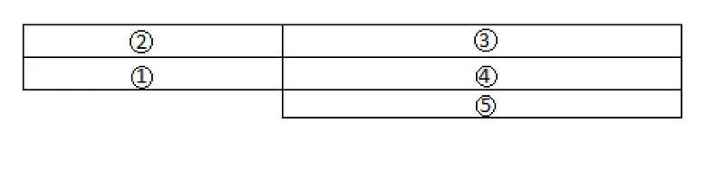
All dimensions are provided in [m] to define the geometry. Hence "convertToMeters" key is set to a value of "1". Vetices are defined as suggested in the first figure. The whole geometry is split into 5 blocks which are defined in the blocks section following the vertices section as suggested in figure 2. Number of elements are set to 200 in x direction and 20 in y direction. Grading is set to (1 1 1) to obtain an uniform mesh for our first simulation.
/*--------------------------------*- C++ -*----------------------------------*\
  =========                 |
  \\      /  F ield         | OpenFOAM: The Open Source CFD Toolbox
   \\    /   O peration     | Website:  https://openfoam.org
    \\  /    A nd           | Version:  9
     \\/     M anipulation  |
\*---------------------------------------------------------------------------*/
FoamFile
{
    format      ascii;
    class       dictionary;
    object      blockMeshDict;
}
// * * * * * * * * * * * * * * * * * * * * * * * * * * * * * * * * * * * * * //

convertToMeters 1;

vertices
(
    (0 0.01 0)		// vertex0
    (0.08 0.01 0)   	// vertex1
    (0.08 0.015 0)	// vertex2
    (0 0.015 0)		// vertex3
    (0.08 0.02 0)	// vertex4
    (0 0.02 0)		// vertex5
    (0.2 0.02 0)	// vertex6
    (0.2 0.015 0)	// vertex7
    (0.2 0.01 0)	// vertex8
    (0.2 0 0)		// vertex9
    (0.08 0 0)		// vertex10

    (0 0.01 0.01)	// vertex11
    (0.08 0.01 0.01)   	// vertex12
    (0.08 0.015 0.01)	// vertex13
    (0 0.015 0.01)	// vertex14
    (0.08 0.02 0.01)	// vertex15
    (0 0.02 0.01)	// vertex16
    (0.2 0.02 0.01)	// vertex17
    (0.2 0.015 0.01)	// vertex18
    (0.2 0.01 0.01)	// vertex19
    (0.2 0 0.01)	// vertex20
    (0.08 0 0.01)	// vertex21

);

blocks
(
    hex (0 1 2 3 11 12 13 14)	//block1
    (80 5 1)
    simpleGrading (1 1 1)

    hex (3 2 4 5 14 13 15 16) 	//block2
    (80 5 1)
    simpleGrading (1 1 1)

    hex (2 7 6 4 13 18 17 15) 	//block3
    (120 5 1)
    simpleGrading (1 1 1)

    hex (1 8 7 2 12 19 18 13) 	//block4
    (120 5 1)
    simpleGrading (1 1 1)

    hex (10 9 8 1 21 20 19 12) 	//block5
    (120 10 1)
    simpleGrading (1 1 1)
);

edges
(
);

boundary
(
    inlet
    {
        type patch;
        faces
        (
            (0 11 14 3)
	    (3 14 16 5)
        );
    }
    outlet
    {
        type patch;
        faces
        (
            (9 8 19 20)
            (8 7 18 19)
	    (7 6 17 18)
        );
    }
    upperWall
    {
        type wall;
        faces
        (
            (5 16 15 4)
            (4 15 17 6)
        );
    }
    lowerWall
    {
        type wall;
        faces
        (
            (0 1 12 11)
            (10 21 12 1)
            (10 9 20 21)
        );
    }
    frontAndBack
    {
        type empty;
        faces
        (
            (0 3 2 1)
            (3 5 4 2)
            (2 4 6 7)
            (1 2 7 8)
            (10 1 8 9)
            (11 12 13 14)
	    (14 13 15 16)
	    (21 20 19 12)
	    (12 19 18 13)
	    (13 18 17 15)
        );
    }
);

// ************************************************************************* //
1b. Material properties, Intial Conditions and Boundary conditions
For current simulation, values of kinematic pressure, p and velocity vector are to be solved in each cell of the discretized domain. Parameter set that would affect the flow in this case are density, velocity, pressure and dynamic viscosity namely `[rho,vecU, p and mu]`. Since density is fixed for incompressible flow the parameter set is reduced to velocity, kinematic pressure and kinematic viscosity - `[vecU, p' and nu]`. Kinematic pressure and kinematic viscosity are obtained by diving pressure and dynamic viscosity by density. Kinematic viscosity can be assumed as constant for our isothermal simulation. Kinematic viscosity is specified in a file named, "transportProperties" inside the folder "constant". This value is kept unchanged for our simulation.
/*--------------------------------*- C++ -*----------------------------------*\
  =========                 |
  \\      /  F ield         | OpenFOAM: The Open Source CFD Toolbox
   \\    /   O peration     | Website:  https://openfoam.org
    \\  /    A nd           | Version:  9
     \\/     M anipulation  |
\*---------------------------------------------------------------------------*/
FoamFile
{
    format      ascii;
    class       dictionary;
    location    "constant";
    object      transportProperties;
}
// * * * * * * * * * * * * * * * * * * * * * * * * * * * * * * * * * * * * * //

nu              [0 2 -1 0 0 0 0] 0.01;


// ************************************************************************* //
Initial and boundary conditions for `vecU and p` are specified in files namely, "U" and "p" present in '0' folder. Our problem is setup using a velocity inlet condition and pressue outlet condition which is recommended for an incompressible flow simulaiton. Velocity at inlet is specified as 1 m/s in x-direction. Reynolds number of the flow at inlet would be calculated using `Re = (Ud)/nu`, where d is hydraulic diameter of inlet. Assuming unit length in z direction for our 2D problem, area of inlet would be `0.01 [m^2]`. Hence `d = 0.1128 [m]` and `Re = 11.28`. This would result in laminar flow. Velocity at outlet is allowed to float using zeroGradient option. Wall are setup using noSlip condition which means 0 velocity at wall. Front and back faces are set as "empty" since we are solving for 2D flow.
Velocity is assumed to be static inside the domain -> (0 0 0) at time = 0.
/*--------------------------------*- C++ -*----------------------------------*\
  =========                 |
  \\      /  F ield         | OpenFOAM: The Open Source CFD Toolbox
   \\    /   O peration     | Website:  https://openfoam.org
    \\  /    A nd           | Version:  9
     \\/     M anipulation  |
\*---------------------------------------------------------------------------*/
FoamFile
{
    format      ascii;
    class       volVectorField;
    object      U;
}
// * * * * * * * * * * * * * * * * * * * * * * * * * * * * * * * * * * * * * //

dimensions      [0 1 -1 0 0 0 0];

internalField   uniform (0 0 0);

boundaryField
{
    inlet
    {
        type            fixedValue;
        value           uniform (1 0 0);
    }

    outlet
    {
        type            zeroGradient;
    }

    upperWall
    {
        type            noSlip;
    }

    lowerWall
    {
        type            noSlip;
    }

    frontAndBack
    {
        type            empty;
    }
}

// ************************************************************************* //
Similarly kinematic pressure at outlet is assumed to be 0. This would result in 0 static pressure at outlet. Pressure at inlet and walls are allowed to float using zeroGradient option.
Pressure is assumed to be 0 at time = 0.
/*--------------------------------*- C++ -*----------------------------------*\
  =========                 |
  \\      /  F ield         | OpenFOAM: The Open Source CFD Toolbox
   \\    /   O peration     | Website:  https://openfoam.org
    \\  /    A nd           | Version:  9
     \\/     M anipulation  |
\*---------------------------------------------------------------------------*/
FoamFile
{
    format      ascii;
    class       volScalarField;
    object      p;
}
// * * * * * * * * * * * * * * * * * * * * * * * * * * * * * * * * * * * * * //

dimensions      [0 2 -2 0 0 0 0];

internalField   uniform 0;

boundaryField
{
    inlet
    {
        type            zeroGradient;
    }

    outlet
    {
        type            fixedValue;
        value           uniform 0;
    }

    upperWall
    {
        type            zeroGradient;
    }

    lowerWall
    {
        type            zeroGradient;
    }

    frontAndBack
    {
        type            empty;
    }
}

// ************************************************************************* //
1c. Solution controls:
Length of the domain is `0.2 [m]`. Using the inlet velocity as average, the flow would approximately take 0.2 [s] to reach the exit. Assuming the flow would reach steady state after 5 flow-throughs, the simulation has to be run for 1 [s]. Using the uniform mesh, the min cell length along x-axis is 0.001 [m]. For explicit simulation, the Courant number criteria has to be less than 1 for the solution to be stable. Using the formula `CFL = (Udt)/dx` and taking `CFL = 1`and `dx = 0.001[m]`, `dt = 0.001 [s]`. Maximum courant number can go beyond 1 where the local velocity is above the inlet velocity. As an inital trial, dt = `0.001 [s]` is used as time-step size and the simulation is run for 1 [s]. These time controls are set in "controlDict" inside "system" folder. Write interval is specified as 100 so that solution data is written out every 0.1 [s] of simulation.
/*--------------------------------*- C++ -*----------------------------------*\
  =========                 |
  \\      /  F ield         | OpenFOAM: The Open Source CFD Toolbox
   \\    /   O peration     | Website:  https://openfoam.org
    \\  /    A nd           | Version:  9
     \\/     M anipulation  |
\*---------------------------------------------------------------------------*/
FoamFile
{
    format      ascii;
    class       dictionary;
    location    "system";
    object      controlDict;
}
// * * * * * * * * * * * * * * * * * * * * * * * * * * * * * * * * * * * * * //

application     icoFoam;

startFrom       startTime;

startTime       0;

stopAt          endTime;

endTime         1;

deltaT          0.001;

writeControl    timeStep;

writeInterval   100;

purgeWrite      0;

writeFormat     ascii;

writePrecision  6;

writeCompression off;

timeFormat      general;

timePrecision   6;

runTimeModifiable true;


// ************************************************************************* //
1d. Solution:
Finite Volume schemes and finite volume solver options specied in "fvSchemes" and "fvSolution" files inside system folder are not altered. Solution is called by issue the command "icoFoam".
Average Courant number during the solution stayed around 0.6 and max Courant number was around 1.6. However the solution remained stable. Number of iterations for `vecU` reduced to 0 after 0.035 [s] of simulation time and number of iterations for `p` reduced to 0 after 0.4 [s] of simulation time. Residuals for both the equations reduced to order of 1e-6 indicating a converged steady solution.
2. Graded mesh:
To study the effects of mesh grading, the test folder cavity is copied to a new folder cavityGrade before the solution step in previous simulation. For control volume method, the flow variables such as velocity and pressure are assumed to be constant within the discretized control volume. Since actual flow might not have same contant values within the control volume, the solution might contain errors. These errors can be reduced by reducing the cell size especially in areas of large gradients of flow variables. When solution variables vary much faster as in the case of boundary layers near walls, multiple cells are required in this region to capture the changes in flow variables. Using a coarse mesh in these areas might introduce errors, which would propogate into the domain. In the current simulation, same number of mesh elements as the previous simulation is used. However the mesh is graded to have finer cells near the wall and coarser cells away from the wall. The mesh grading factor is taken to be 0.2 for this simulation. This means that the smallest cell in the block is 20% of the largest cell in the block. "blockMeshDict" inside systems folder is modified to create a graded mesh with finer mesh elements near the wall.
/*--------------------------------*- C++ -*----------------------------------*\
  =========                 |
  \\      /  F ield         | OpenFOAM: The Open Source CFD Toolbox
   \\    /   O peration     | Website:  https://openfoam.org
    \\  /    A nd           | Version:  9
     \\/     M anipulation  |
\*---------------------------------------------------------------------------*/
FoamFile
{
    format      ascii;
    class       dictionary;
    object      blockMeshDict;
}
// * * * * * * * * * * * * * * * * * * * * * * * * * * * * * * * * * * * * * //


convertToMeters 1;

vertices
(
    (0 0.01 0)		// vertex0
    (0.08 0.01 0)   	// vertex1
    (0.08 0.015 0)	// vertex2
    (0 0.015 0)		// vertex3
    (0.08 0.02 0)	// vertex4
    (0 0.02 0)		// vertex5
    (0.2 0.02 0)	// vertex6
    (0.2 0.015 0)	// vertex7
    (0.2 0.01 0)	// vertex8
    (0.2 0 0)		// vertex9
    (0.08 0 0)		// vertex10

    (0 0.01 0.01)	// vertex11
    (0.08 0.01 0.01)   	// vertex12
    (0.08 0.015 0.01)	// vertex13
    (0 0.015 0.01)	// vertex14
    (0.08 0.02 0.01)	// vertex15
    (0 0.02 0.01)	// vertex16
    (0.2 0.02 0.01)	// vertex17
    (0.2 0.015 0.01)	// vertex18
    (0.2 0.01 0.01)	// vertex19
    (0.2 0 0.01)	// vertex20
    (0.08 0 0.01)	// vertex21

);

blocks
(
    hex (0 1 2 3 11 12 13 14)	//block1
    (80 5 1)
    simpleGrading (0.2 5 1)

    hex (3 2 4 5 14 13 15 16) 	//block2
    (80 5 1)
    simpleGrading (0.2 0.2 1)

    hex (2 7 6 4 13 18 17 15) 	//block3
    (120 5 1)
    simpleGrading (5 0.2 1)

    hex (1 8 7 2 12 19 18 13) 	//block4
    (120 5 1)
    simpleGrading (5 5 1)

    hex (10 9 8 1 21 20 19 12) 	//block5
    (120 10 1)
    simpleGrading (5 0.2 1)
);

edges
(
);

boundary
(
    inlet
    {
        type patch;
        faces
        (
            (0 11 14 3)
	    (3 14 16 5)
        );
    }
    outlet
    {
        type patch;
        faces
        (
            (9 8 19 20)
            (8 7 18 19)
	    (7 6 17 18)
        );
    }
    upperWall
    {
        type wall;
        faces
        (
            (5 16 15 4)
            (4 15 17 6)
        );
    }
    lowerWall
    {
        type wall;
        faces
        (
            (0 1 12 11)
            (10 21 12 1)
            (10 9 20 21)
        );
    }
    frontAndBack
    {
        type empty;
        faces
        (
            (0 3 2 1)
            (3 5 4 2)
            (2 4 6 7)
            (1 2 7 8)
            (10 1 8 9)
            (11 12 13 14)
	    (14 13 15 16)
	    (21 20 19 12)
	    (12 19 18 13)
	    (13 18 17 15)
        );
    }
);

// ************************************************************************* //
Initial conditions and boundary conditions are left as same used for previous simulation. The time step size has to be modified to the current mesh. The smallest mesh length along x-axis is found to be 0.0004 [m] by opening the mesh in paraFoam and coloring the boundaries using face-area magnitude. Hence, to obtain CFL number of 1 and having velocity U = 1 m/s, time-step size should be 0.0004 [s]. However, the simulation using time-step size of 0.0004 [s] diverges since local CFL number is larger than 1 due to local velocities exceeding the inlet velocity. By reducing the time-step size in stages, the simulation was found to be stable at 0.0001 [m]. "controlDict" is modifed to use this time-step size. Write interval is updated to 1000 to write the solution every 0.1 [s] of simulaiton time.
/*--------------------------------*- C++ -*----------------------------------*\
  =========                 |
  \\      /  F ield         | OpenFOAM: The Open Source CFD Toolbox
   \\    /   O peration     | Website:  https://openfoam.org
    \\  /    A nd           | Version:  9
     \\/     M anipulation  |
\*---------------------------------------------------------------------------*/
FoamFile
{
    format      ascii;
    class       dictionary;
    location    "system";
    object      controlDict;
}
// * * * * * * * * * * * * * * * * * * * * * * * * * * * * * * * * * * * * * //

application     icoFoam;

startFrom       startTime;

startTime       0;

stopAt          endTime;

endTime         1;

deltaT          0.0001;

writeControl    timeStep;

writeInterval   1000;

purgeWrite      0;

writeFormat     ascii;

writePrecision  6;

writeCompression off;

timeFormat      general;

timePrecision   6;

runTimeModifiable true;


// ************************************************************************* //
Finite volume schemes and solver options are left as same for previous simulation. The solver is called by issuing "icoFoam" command. Average CFL number is around 0.06 and max CFL number is around 0.36.
Results:
Results for both the simulations are compared using paraFoam. A slice is created at mid-Z section and colored by velocity. A line parallel to Y-axis is created and x-velocity is plotted along this line for both the simulations
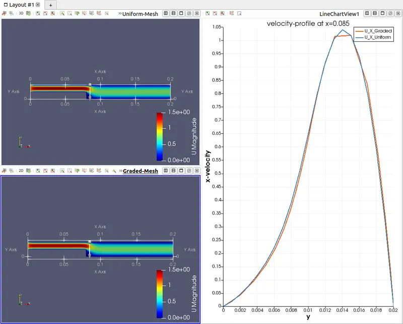
First and second contour on the left side of the image show the contour plots of velocity magnitude on the clip plane. The downward arrow shows the position of the line on which the scatter plot of x-velocity is generated on the right. The contour plots doesn't show much difference in the flow pattern. However considerable difference is seen in the xy-plot, especially at the velocity peak, y = 0.014 [m]. The graded mesh seems to have under-resolved the velocity profile, loosing the velocity peak. This could be due to the fact that the mesh is refined along the wall, y = 0, 0.01 and 0.02 [m]. This would cause coarser mesh to be formed at y = 0.014 [m], hence under-resolving the flow. When gradients of flow parameters such as the velocity peak in above picture, sufficient number of cells are required to capture the profile correctly. Lower cell count could lead to under-resolved profiles such as with the graded mesh. However, grading is recommended near the walls to capture velocity profiles accurately. In the current case, the total number of cells used is insufficient to obtain a grid independent result. With increased cell count, the velocity profile would be captured smoothly with the peak. The use of graded mesh is not apparant in this study. Not much difference in velocity profile is seen near the walls, perhaps due to the lower Reynolds number of the flow. With large reynolds number flows, the boundary layers are much shorted and velocity gradients would be much steeper requiring large number of cells to capture the profile accurately. In such cases, the use of graded mesh would be apparant. In flows involving shock waves, similar steep gradients of flow variables can be seen across shock waves. In such cases as well, mesh is required to be refined along the shock waves to obtain good results. In cases, where the location of steep gradients of flow variables could not be predicted, such as in the current simulation with velocity peak occurring at y = 0.014 [m], a grid independent study or dynamic mesh adaption is required to capture the gradients correcly.