Week 3.5 - Deriving 4th order approximation of a 2nd order derivative using Taylor Table method
Derive the following 4th order approximations of the second-order derivative.
1. Central difference
Based on hint (i), central difference scheme for second order derivative will need 5 nodes in the numerical stencil to get an order of accuracy of 4.
`P = N - Q + 1`
P = 4, Q = 2. Therefore N = 5
Formulating discretized numerial equation using 5 nodes:
`f''(x) = af(i-2) + bf(i-1) + cf(i) + df(i+1)+ef(i+2)` ---- (1)
Taylor series is formed for the terms in equ (1)
5 terms are used in the series to form 5 equations to obtain the 5 unknowns --> [a b c d e]
`af(i-2) = a(f(i) - (f'(i) 2Deltax)/(1!) + (f''(i)(2Deltax)^2)/(2!) - (f'''(i)(2Deltax)^3)/(3!) + (f^(iv)(i)(2Deltax)^4)/(4!))`
`bf(i-1) = b(f(i) - (f'(i) Deltax)/(1!) + (f''(i)(Deltax)^2)/(2!) - (f'''(i)(Deltax)^3)/(3!) + (f^(iv)(i)(Deltax)^4)/(4!))`
`cf(i) = cf(i)`
`df(i+1) = d(f(i) + (f'(i) Deltax)/(1!) + (f''(i)(Deltax)^2)/(2!) + (f'''(i)(Deltax)^3)/(3!) + (f^(iv)(i)(Deltax)^4)/(4!))`
`ef(i+2) = e(f(i) + (f'(i) 2Deltax)/(1!) + (f''(i)(2Deltax)^2)/(2!) + (f'''(i)(2Deltax)^3)/(3!) + (f^(iv)(i)(2Deltax)^4)/(4!))`
Taylor table is formed using coefficients of the common terms in above Taylor series equations
| Terms in equ (1) | `f(i)` | `Deltax f'(i)` | `Deltax^2 f''(i)` | `Deltax^3 f'''(i)` | `Deltax^4 f^(iv)(i)` |
| `af(i-2)` | a | -2a | 4a/2 | -8a/6 | 16a/24 |
| `bf(i-1)` | b | -b | b/2 | -b/6 | b/24 |
| `cf(i)` | c | 0 | 0 | 0 | 0 |
| `df(i+1)` | d | d | d/2 | d/6 | d/24 |
| `ef(i+2)` | e | 2e | 4e/2 | 8e/6 | 16e/24 |
| Total | 0 | 0 | `1/(Deltax)^2` | 0 | 0 |
Final row(Total) values are defined such that, summation of all terms in the Taylor series expansion results in `f''(x)`
Provided individual equaitons for each column, values for [a b c d e] can be determined.
`a + b + c + d + e = 0`
`-2a - b + d + 2e = 0`
`(4a)/2 + b/2 + d/2 + (4e)/2 = 1/(Deltax)^2 ` --> `4a + b + d + 4e = 2/(Deltax)^2`
`-(8a)/6 - b/6 + d/6 + (8e)/6 = 0` --> `-8a - b + d + 8e = 0`
`(16a)/24 + b/24 + d/24 + (16e)/24 = 0` --> `16a + b + d + 16e = 0`
Solving for the variables above:
`a = -5/(60*Deltax^2); b = 4/(3*Deltax^2); c = -5/(2*Deltax^2); d = 4/(3*Deltax^2); e = -5/(60*Deltax^2)`
`f''(x) = (-5/60 f(i-2) + 4/3 f(i-1) - 5/2 f(i) + 4/3 f(i+1)- 5/60 f(i+2))/(Deltax)^2`
2. Skewed right-sided difference
Based on hint (ii), central difference scheme for second order derivative will need 5 nodes in the numerical stencil to get an order of accuracy of 4.
`P = N - Q`
P = 4, Q = 2. Therefore N = 6
Formulating discretized numerial equation using 5 nodes:
`f''(x) = af(i) + bf(i+1) + cf(i+2) + df(i+3) + ef(i+4) + gf(i+5)` ---- (2)
Taylor series is formed for the terms in equ (2)
6 terms are used in the series to form 6 equations to obtain the 6 unknowns --> [a b c d e g]
`af(i) =af(i)`
`bf(i+1) = b(f(i) + (f'(i) Deltax)/(1!) + (f''(i)(Deltax)^2)/(2!) + (f'''(i)(Deltax)^3)/(3!) + (f^(iv)(i)(Deltax)^4)/(4!) + (f^(v)(i)(Deltax)^5)/(5!))`
`cf(i+2) = c(f(i) + (f'(i) 2Deltax)/(1!) + (f''(i)(2Deltax)^2)/(2!) + (f'''(i)(2Deltax)^3)/(3!) + (f^(iv)(i)(2Deltax)^4)/(4!) + (f^(v)(i)(2Deltax)^5)/(5!))`
`df(i+3) = d(f(i) + (f'(i) 3Deltax)/(1!) + (f''(i)(3Deltax)^2)/(2!) + (f'''(i)(3Deltax)^3)/(3!) + (f^(iv)(i)(3Deltax)^4)/(4!) + (f^(v)(i)(3Deltax)^5)/(5!))`
`ef(i+4) = e(f(i) + (f'(i) 4Deltax)/(1!) + (f''(i)(4Deltax)^2)/(2!) + (f'''(i)(4Deltax)^3)/(3!) + (f^(iv)(i)(4Deltax)^4)/(4!) + (f^(v)(i)(4Deltax)^5)/(5!))`
`gf(i+5) = g(f(i) + (f'(i) 5Deltax)/(1!) + (f''(i)(5Deltax)^2)/(2!) + (f'''(i)(5Deltax)^3)/(3!) + (f^(iv)(i)(5Deltax)^4)/(4!) + (f^(v)(i)(5Deltax)^5)/(5!))`
Taylor table is formed using coefficients of the common terms in above Taylor series equations
| Terms in equ (1) | `f(i)` | `Deltax f'(i)` | `Deltax^2 f''(i)` | `Deltax^3 f'''(i)` | `Deltax^4 f^(iv)(i)` | `Deltax^5 f^(v)(i)` |
| `af(i)` | a | 0 | 0 | 0 | 0 | 0 |
| `bf(i+1)` | b | b | b/2 | b/6 | b/24 | b/120 |
| `cf(i+2)` | c | 2c | 4c/2 | 8c/6 | 16c/24 | 32c/120 |
| `df(i+3)` | d | 3d | 9d/2 | 27d/6 | 81d/24 | 243d/120 |
| `ef(i+4)` | e | 4e | 16e/2 | 64e/6 | 256e/24 | 1024e/120 |
| `gf(i+4)` | g | 5g | 25g/2 | 125g/6 | 625g/24 | 3125g/120 |
| Total | 0 | 0 | `1/(Deltax)^2` | 0 | 0 | 0 |
Final row(Total) values are defined such that, summation of all terms in the Taylor series expansion results in `f''(x)`
Provided individual equaitons for each column, values for [a b c d e g] can be determined.
`a + b + c + d + e + g = 0`
`b + 2c + 3d + 4e + 5g = 0`
`b/2 + (4c)/2 + (9d)/2 + (16e)/2 + (25g)/2 = 1/(Deltax)^2` --> `b + 4c + 9d +16e + 25g = 2/(Deltax)^2`
`b/6 + (8c)/6 + (27d)/6 + (64e)/6 + (125g)/6= 0` --> `b + 8c + 27d + 64e + 125g = 0`
`b/24 + (16c)/24 + (81d)/24 + (256e)/24 + (625g)/24= 0` --> `b + 16c + 81d + 256e + 625g = 0`
`b/120 + (32c)/120 + (243d)/120 + (1024e)/120 + (3125g)/120= 0` --> `b + 32c + 243d + 1024e + 3125g = 0`
Solving for the variables above:
`a = 15/(4*Deltax^2); b = -77/(6*Deltax^2); c = 107/(6*Deltax^2); d = -13; e = 61/(12*Deltax^2); g = -5/(6*Deltax^2)`
Equ (2) becomes
`f''(x) = (15/4 f(i) - 77/6 f(i+1) + 107/6 f(i+2) - 13 f(i+3) + 61/12 f(i+4) - 5/6 f(i+5))/(Deltax)^2`
Order of numerical scheme:
For Taylor series expansion of the terms in equ (2), the first term ignored is the sixth order derivative term.
Let the summation of equations for expansion of RHS of equ(2) using Taylor series be Z.
Including the ignored term in equ (2)
`f''(x) = Z + b(f^(vi)(i)(Deltax)^6)/(6!) + c(f^(vi)(i)(2Deltax)^6)/(6!) + d(f^(vi)(i)(3Deltax)^6)/(6!) + e(f^(vi)(i)(4Deltax)^6)/(6!) + g(f^(vi)(i)(5Deltax)^6)/(6!)`
Taking out the common terms
`f''(x) = Z + (f^(vi)(i)Deltax^6)/(6!)(b + 2^6c + 3^6d + 4^6e + 5^6g)`
`b + 2^6c + 3^6d + 4^6e + 5^6g != 0`
`(f^(vi)(i)Deltax^6)/(6!)(b + 2^6c + 3^6d + 4^6e + 5^6g) != 0`
Hence ignoring this term will cause error in solution for f''(x).
The order of this error can be determined by providing a general form for the coefficients [b c d e g]
[b c d e g] will be in the form `C_1/(Deltax)^2` --> where `C_1` is a constant
Hence, `b + 2^6c + 3^6d + 4^6e + 5^6g = C_2/(Deltax)^2` --> where `C_2` is a constant
The ignored term then becomes
`(f^(vi)(i)Deltax^6)/(6!)(b + 2^6c + 3^6d + 4^6e + 5^6g) = (f^(vi)(i)Deltax^6)/(6!) C_2/(Deltax)^2`
With further simplification the term becomes
`C * f^(vi)(i) * Deltax^4` --> where C is a constant
Hence the ignored term is of order `Deltax^4` or 4th order
3. Skewed left-sided difference
Based on hint (ii), central difference scheme for second order derivative will need 5 nodes in the numerical stencil to get an order of accuracy of 4.
`P = N - Q`
P = 4, Q = 2. Therefore N = 6
Formulating discretized numerial equation using 5 nodes:
`f''(x) = af(i) + bf(i-1) + cf(i-2) + df(i-3) + ef(i-4) + gf(i-5)` ---- (3)
Taylor series is formed for the terms in equ (3)
6 terms are used in the series to form 6 equations to obtain the 6 unknowns --> [a b c d e g]
`af(i) =af(i)`
`bf(i-1) = b(f(i) - (f'(i) Deltax)/(1!) + (f''(i)(Deltax)^2)/(2!) - (f'''(i)(Deltax)^3)/(3!) + (f^(iv)(i)(Deltax)^4)/(4!) - (f^(v)(i)(Deltax)^5)/(5!))`
`cf(i-2) = c(f(i) - (f'(i) 2Deltax)/(1!) + (f''(i)(2Deltax)^2)/(2!) - (f'''(i)(2Deltax)^3)/(3!) + (f^(iv)(i)(2Deltax)^4)/(4!) - (f^(v)(i)(2Deltax)^5)/(5!))`
`df(i-3) = d(f(i) - (f'(i) 3Deltax)/(1!) + (f''(i)(3Deltax)^2)/(2!) - (f'''(i)(3Deltax)^3)/(3!) + (f^(iv)(i)(3Deltax)^4)/(4!) - (f^(v)(i)(3Deltax)^5)/(5!))`
`ef(i-4) = e(f(i) - (f'(i) 4Deltax)/(1!) + (f''(i)(4Deltax)^2)/(2!) - (f'''(i)(4Deltax)^3)/(3!) + (f^(iv)(i)(4Deltax)^4)/(4!) - (f^(v)(i)(4Deltax)^5)/(5!))`
`gf(i-5) = g(f(i) - (f'(i) 5Deltax)/(1!) + (f''(i)(5Deltax)^2)/(2!) - (f'''(i)(5Deltax)^3)/(3!) + (f^(iv)(i)(5Deltax)^4)/(4!) - (f^(v)(i)(5Deltax)^5)/(5!))`
Taylor table is formed using coefficients of the common terms in above Taylor series equations
| Terms in equ (1) | `f(i)` | `Deltax f'(i)` | `Deltax^2 f''(i)` | `Deltax^3 f'''(i)` | `Deltax^4 f^(iv)(i)` | `Deltax^5 f^(v)(i)` |
| `af(i)` | a | 0 | 0 | 0 | 0 | 0 |
| `bf(i+1)` | b | -b | b/2 | -b/6 | b/24 | -b/120 |
| `cf(i+2)` | c | -2c | 4c/2 | -8c/6 | 16c/24 | -32c/120 |
| `df(i+3)` | d | -3d | 9d/2 | -27d/6 | 81d/24 | -243d/120 |
| `ef(i+4)` | e | -4e | 16e/2 | -64e/6 | 256e/24 | -1024e/120 |
| `gf(i+4)` | g | -5g | 25g/2 | -125g/6 | 625g/24 | -3125g/120 |
| Total | 0 | 0 | `1/(Deltax)^2` | 0 | 0 | 0 |
Final row(Total) values are defined such that, summation of all terms in the Taylor series expansion results in `f''(x)`
Provided individual equaitons for each column, values for [a b c d e g] can be determined.
`a + b + c + d + e + g = 0`
`-b - 2c - 3d - 4e - 5g = 0`
`b/2 + (4c)/2 + (9d)/2 + (16e)/2 + (25g)/2 = 1/(Deltax)^2` --> `b + 4c + 9d +16e + 25g = 2/(Deltax)^2`
`-b/6 - (8c)/6 - (27d)/6 - (64e)/6 - (125g)/6= 0` --> `-b - 8c - 27d - 64e - 125g = 0`
`b/24 + (16c)/24 + (81d)/24 + (256e)/24 + (625g)/24= 0` --> `b + 16c + 81d + 256e + 625g = 0`
`-b/120 - (32c)/120 - (243d)/120 - (1024e)/120 - (3125g)/120= 0` --> `-b - 32c - 243d - 1024e - 3125g = 0`
Solving for the variables above:
`a = 15/(4*Deltax^2); b = -77/(6*Deltax^2); c = 107/(6*Deltax^2); d = -13; e = 61/(12*Deltax^2); g = -5/(6*Deltax^2)`
Equ (3) becomes
`f''(x) = (15/4 f(i) - 77/6 f(i+1) + 107/6 f(i+2) - 13 f(i+3) + 61/12 f(i+4) - 5/6 f(i+5))/(Deltax)^2`
Order of numerical scheme:
The order of this scheme will also be of fourth order and the derivation of this error term is exactly same as for forward skewed approximation.
Matlab program:
1. A helper function is created to calculate f(x) when x is provided
function fx = fx_calc(x)
%   calculate f(x) for given value of x
fx = exp(x) * cos(x);
end
2. A central diferncing scheme funtion is created to calcuate f''(x) when the coefficient array, x and dx are provided.
A numeical stencil is created using x and dx values.
Then central differencing approximation equation is applied using the provided values for coefficients
function f_double_dash_x = centralDifference(a,x,dx)
% Caculate f''(x) using central difference numerical
% scheme with 4th order accuracy

% define numerical stencil
stencil = [x-2*dx; x-dx; x; x+dx; x+2*dx];

% f(x) is calculated for all values of x in stencil
fx = arrayfun(@fx_calc,stencil);

% calculate f''(x) using the central differencing scheme
% Deltax^2 is divided finally in f''(x) calculation to account
% for coefficient array ignoring this term
f_double_dash_x =  sum(a .* fx)/dx^2;
end
3.Similarly, forward skewed and backward skewed functions are implemented
function f_double_dash_x = forwardDifference(a,x,dx)
% Caculate f''(x) using central difference numerical
% scheme with 4th order accuracy

% define numerical stencil
stencil = [x; x+dx; x+2*dx; x+3*dx; x+4*dx; x+5*dx];

% f(x) is calculated for all values of x in stencil
fx = arrayfun(@fx_calc,stencil);

% calculate f''(x) using the central differencing scheme
% Deltax^2 is divided finally in f''(x) calculation to account
% for coefficient array ignoring this term
f_double_dash_x =  sum(a .* fx)/dx^2;
end
function f_double_dash_x = backwardDifference(a,x,dx)
% Caculate f''(x) using central difference numerical
% scheme with 4th order accuracy
% define numerical stencil
stencil = [x; x-dx; x-2*dx; x-3*dx; x-4*dx; x-5*dx];
% f(x) is calculated for all values of x in stencil
fx = arrayfun(@fx_calc,stencil);
% calculate f''(x) using the central differencing scheme
% Deltax^2 is divided finally in f''(x) calculation to account
% for coefficient array ignoring this term
f_double_dash_x = sum(a .* fx)/dx^2;
end4.The main function included the values for x and dx. dx is defined as a array of 500 values between pi/2000 and pi/20. x as pi/2
Analytical result is calculated using second derivative of the function
For each differencing scheme, the set of equations are defined in matrix terms, A x coeff = b.
b array ignores the `1/(Deltax)^2` term. This term is in turn used to divide the final result for f''(x) in the functions defined above.
Looping over values of dx, f''(x) and it's absolute error with respect to analytical result is calculated for all the 3 schemes.
Finally the errors are ploted against dx in loglog plot.
clear all
close all
clc

% function f(x) = exp(x) * cos(x)

% Define input varibles
x = pi/2;
dx = linspace(pi/2000,pi/20,500);

% Analytical solution
% f'(x) = -exp(x) * (sin(x) - cos(x))
% f''(x) = -2*exp(x)*sin(x)
analyticalResult = -2*exp(x)*sin(x);

% Numerical solution
% Define set of equations from the derived
% numerical schemes for 4th order approximation

% Central difference scheme
% Set of linear equations defined using matrices -> A*coeff = b
A_central_diff = [1 1 1 1 1;
                -2 -1 0 1 2;
                 4 1 0 1 4;
                -8 -1 0 1 8;
                16 1 0 1 16];

% b defined as RHS of system of equation ignoring the 1/Deltax^2 term
b_central_diff = [0; 0; 2; 0; 0];

% coefficient array is defined as [a b c d e] / (Deltax)^2
% Deltax^2 will be divided finally in f''(x) calculation
coeff_central_diff =  A_central_diff\b_central_diff;

% calculate f''(x) using different values of dx
centralDifference_result = zeros(1, length(dx));
centralDifference_error = zeros(1, length(dx));
for i  = 1:length(dx)
    centralDifference_result(i) = centralDifference(coeff_central_diff,x,dx(i));
    centralDifference_error(i) = abs(analyticalResult - centralDifference_result(i));
end

% Forward skewed difference scheme
A_forward_diff = [1 1 1 1 1 1;
                  0 1 2 3 4 5;
                  0 1 4 9 16 25;
                  0 1 8 27 64 125;
                  0 1 16 81 25 625;
                  0 1 32 243 1024 3125];

% b deined as RHS of system of equation ignoring the 1/Deltax^2 term
b_forward_diff = [0; 0; 2; 0; 0; 0];

% coefficient array is defined as [a b c d e] / (Deltax)^2
% Deltax^2 will be divided finally in f''(x) calculation
coeff_forward_diff =  A_forward_diff\b_forward_diff;

% calculate f''(x) using different values of dx
forwardDifference_result = zeros(1, length(dx));
forwardDifference_error = zeros(1, length(dx));
for i  = 1:length(dx)
    forwardDifference_result(i) = forwardDifference(coeff_forward_diff,x,dx(i));
    forwardDifference_error(i) = abs(analyticalResult - forwardDifference_result(i));
end

% Backward skewed difference scheme
A_backward_diff = [1 1 1 1 1 1;
                  0 -1 -2 -3 -4 -5;
                  0 1 4 9 16 25;
                  0 -1 -8 -27 -64 -125;
                  0 1 16 81 25 625;
                  0 -1 -32 -243 -1024 -3125];

% b deined as RHS of system of equation ignoring the 1/Deltax^2 term
b_backward_diff = [0; 0; 2; 0; 0; 0];

% coefficient array is defined as [a b c d e] / (Deltax)^2
% Deltax^2 will be divided finally in f''(x) calculation
coeff_backward_diff =  A_backward_diff\b_backward_diff;

% calculate f''(x) using different values of dx
backwardDifference_result = zeros(1, length(dx));
backwardDifference_error = zeros(1, length(dx));
for i  = 1:length(dx)
    backwardDifference_result(i) = backwardDifference(coeff_backward_diff,x,dx(i));
    backwardDifference_error(i) = abs(analyticalResult - backwardDifference_result(i));
end

loglog(dx,centralDifference_error)
hold on
loglog(dx,forwardDifference_error)
loglog(dx,backwardDifference_error)
legend("centralDifference error","forwardDifference error","backwardDifference error")
legend("Location","best")
xlabel("dx(log scale)")
ylabel("absolute difference(log scale)")
5.Result:
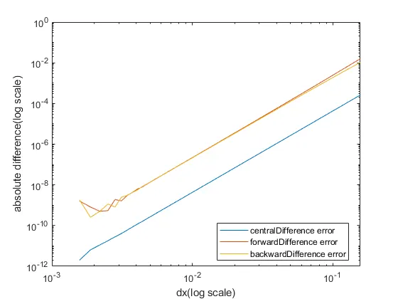
6.Results show all the 3 schemes have similar slope on log plot meaning they have same order of acuracy.
However the absolute error is less for central difference scheme compared to the skewed difference schemes.
Skewed difference schmes will be useful when the defined function is valid only for a particular range of x.
Values of f'(x) or f''(x) at boundary values of x cannot be calculated using central difference equations since, f(x-dx) or f(f+dx) is undefined.