Week 9 - FVM Literature Review

1. Finite Volume Method(FVM):

FVM is a method of discretizing partial differential governing equation of fluid flow into numerical algebraic equations. The domain, where the solution of partial differential equations are to be obtained, is split into multiple finite volumes. The finite volumes could be of any arbitrary shape, which makes it the most preferable solution technique in CFD industry. The partial differential governing equations are converted to integral form. Volume integral terms in those equations are converted to surface integrals using divergence theorem. Integral forms of the governing equations are then applied to each of the control volumes. The surface integrals are calculated using a simple summation over the faces that form the control volume. An implicit assumption, that the flow variables and their derivatives are contant on each face of the control volume is made to calculate the summation. Face center values of terms included in surface intergral are calculated using a suitable interpolation scheme from the neighboring cell center values. Hence, algrebraic equations are formed for each partial differential governing equation at cell centroids of interior cells. With boundary conditions applied on exterior cells, N number of algebraic equations are formed for N number of cells in the domain. A suitable iterative scheme can be employed similar to Finite Difference Method(FDM) to solve for the primitive variables at each cell centroid.

2. Major differences between Finite Volume Method(FVM) and Finite Difference Method(FDM):

FVM	FDM
Domain is discretized into finite volumes. Primitve variables are calculated at cell centroids.	Domain in discretized into finite number of points. Primitive variables are calculated at the discrete points.
Finite volumes could be formed of any artibrary shape. To calculate derivatives in global coordinate directions, rather simple corrections could be applied to interpolation schemes when the cells are not aligned in primary/secondary axes.	Discrete points are preferred to be aligned with primary/seconary axes to calculate the derivatives in global coordinate directions. Trasformation schemes might need to be applied when the points are not aligned to be able to calculate the solution on an alternative aligned grid and transform it back to the original domain. The process is tedius for complex geometries.
Integral forms of conservation governing equations are applied on control volumes to obtain the solution on cell centroids. This preserves the conservative property in each cell and hence the whole domain.	Partial differential governing equations are directly applied on the discrete points and hence this scheme is generally non-conservative for non-linear solutions until convergence is obtained.
The governing equations depends on source terms in the cell and fluxes of properties through faces. So, face centroid properties and derivatives are required. These are obtained through suitable derivative and interpolation schemes. The order of accuracy depends on these derivative and interpolaiton schemes.	Truncated taylor series approximation is used to calculate the derivative terms in the governing equations. The order of accuracy depends on the truncation error in taylor series approximation.

3. Solving 1D heat conduction equation using FVM:

1D steady heat conduction equation in partial differential form is given by:

`del/(delx)(alpha (delT)/(delx)) + S_T = 0`

where `S_T` -> thermal source term, which could be a function of thermal properties and local temperature.

and `alpha` -> thermal diffusivity of the material, which could be approximated as a constant or as a function of local temperature

In FDM, this equation is directly applied on discrete points on the domain. The derivatives are approximated using truncated taylor series and expressions for temperature at the points are formed as ordinary algebraic equations.

3a. Domain discretization:

In FVM though, the domain is approximated as control volumes as shown below. The top and bottom faces of the volumes are represented by dotted lines. Since we are solving for 1D problem, the control volumes are represented by the line segments between the divinding lines and cell centroid would be the midpoint of these line segments. For 2D problems, control volumes would be formed by 2 dimensional faces and cell centroids would be represented by the face centroid. 3D problems would have faces in all directions forming a proper 3 dimensional volume and cell centroid would be the volume centroid.

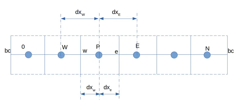
Here 1D line segment is divided into N+1 cells with 0 and N representing exterior boundary cells. For interior cell, an algebraic equation is generated from the integral form of governing equation. Let's consider for example, the cell "P". West and east side cell centroid are marked by "W" and "E" respectively. West and east faces forming the cell "P" are marked by "w" and "e" respectively. The cell centroid "P" is `dx_w` and `dx_e` distance away from the face centroids on west and east faces respectively. Similarly, "P" is away from west and east cell centroids by a distance of `dx_W` and `dx_E` respectively. For boundary cells similar equations could be formed using the knowledge of primitive variables or it's derivaties at the boundary faces, marked as "bc"

3b. Governing equation discretization:

Next step is discretize the partial differential governing equation in algebraic form so as to apply the interative solution technique. Integrating the differential governing equation over a control volume, suppose "P" will result in

`int_v del/(delx)(alpha(delT)/(delx))dv + int_vS_Tdv = 0`

This can be written in divergence of vector form in 1D using `veci` which represents unit vector in x direction.

`int_v nabla.(alpha (delT)/(delx)veci)dv + int_vS_Tdv = 0`

Applying Gauss divergence theorem, the volume integral for diffusion term can be converted to surface integral form

`int_s alpha (delT)/(delx)veci . vec(dS) + int_vS_Tdv = 0`

where, `vec(dS)` -> normal surface vector of the control volume

Surface integral term could be calculated using a simple summation of `(alpha (delT)/(delx))` over the faces by assuming `alpha` and `(delT)/(delx)` as constant over individual faces.

`int_s alpha (delT)/(delx)veci . vec(dS) = sum_(n = e,w)alpha (delT)/(delx)veci.vecA= (alpha(delT)/(delx)A)_e - (alpha(delT)/(delx)A)_w`

where A -> surface area of the face. The term for west face becomes negative since the area vector points in negative x direction, i.e., `-veci`

Interpolation Schemes:

`alpha, (delT)/(delx) and A` have to be obtained at face centroids of the surrounding faces of the control volume, namely "e" and "w" in this case. `alpha` at face centroid could be obtained from material properties if a constant approximation is made. Else, this value can be obtained using interpolation schemes based on adjacent cell center values when it's a function of primary variable. Various interpolation schemes are available to for this purpose. One such simple interpolation scheme is linear interpolation.

`alpha_e = dx_e/dx_E alpha_p + (1 - dx_e/dx_E)alpha_E`

`alpha_w = dx_w/dx_W alpha_p + (1 - dx_w/dx_W)alpha_W`

Similarly, various gradient schemes are available to calculate `(delT)/(delx)` at face centroid based on adjacent cell centroid values. Using linear interpolation between the adjacent cell centroids, these could be calculated using following formulas

`((delT)/(delx))_e = (T_E - T_P)/dx_E`

`((delT)/(delx))_w = (T_P - T_W)/dx_W`

Some of the common interpolation schemes used for determining a variable at the face centroid include:

i. Linear / Central differencing

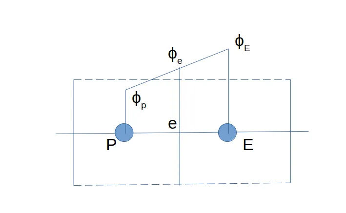
A linear profile of the variable is assumed between the cell centroids. Value of face centroid is obtained using cell centroid values of adjacent cells as shown above. This provides a second order accuracy. But due to unboundedness, this method could sometimes lead to instability in solution. `phi` represent solution variable in the following image.

i. Upwind / First order upwind

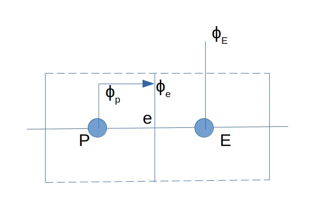
The face center value of a variable is approximated as its cell center value. This scheme is first order accurate but provides high stability to the solution.

iii. second order upwind

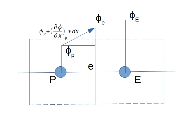
Derivative of the variable at cell center and distance to the face centroid are used to calculate the change of `phi` until face centroid. This value is then added to cell centroid value of the variable to obtain the face center value of `phi`. This scheme is also second order accurate and reasonably stable. However, it involves additional calculation of derivative of variables at cell center based on neighboring cells.

iv. QUICK:

QUICK scheme uses 3 cell center values of `phi`, 2 upstream and 1 downstream to calculate the value of `phi` at the face centroid using a quadratic variation assumption. This scheme is third order accurate for uniform mesh.

Flux limiters:

Derivates of variables are required at cell centers when using schemes such as linear upwind scheme. Based on these derivatives `phi` is calculated on face centers. Sometimes, these derivatives are very large, such as near shock waves. These could lead to values of `phi` at faces to be greater than the neighboring cell center values. This overshooting can lead to solution instabilities and oscillation in solution when using higher order schemes. A scenario where `((delphi)/(delx))_p` is very large causing `phi_e` to overshoot is shown below.

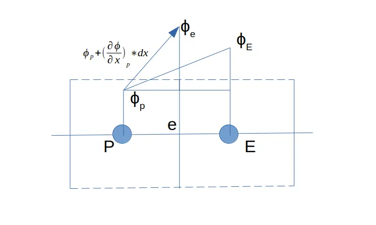
In such cases, a limiter function is necessary to limit the gradient at "p" to a value acceptable by the neighbouring cells.

`phi_e = phi_p + psi*((delphi)/(delx))_p dx_e`, `0 <=psi <= 1`

where `psi` -> slope limiter to limit the gradient term such that `psi` value at face doesn't overshoot the neighbouring cell center when the gradient is positive and `psi` value doesn't undershoot the neighbouring cell center when gradient is negative.

In general terms, the flux or variable `phi` at face center is calculated using

`phi = phi_l + psi * (phi_h - phi_l)` ,

where `phi_l` -> face center value calculated using lower order scheme

`phi_h` -> face center value calculated using higher order scheme

and `psi`-> flux limiter, calculated as a function of ratio of slopes at cell center calculated using backward and forward differencing.

Hence, the flux limiter scheme takes advantage of stability offered by lower order interpolation and accuracy provided by higher order interpolation to maintain the fluxes and primitive variables in physically acceptable range.

3c. Solution using algebraic equation:

The integral form of governing equation can now be converted to algebraic form using the above discretization as

`int_s alpha (delT)/(delx)veci . vec(dS) + int_vS_Tdv = 0`

`alpha_e(T_E - T_P)/dx_EA_e - alpha_w(T_P - T_W)/dx_WA_w + bar(S_T)dv = 0`

where, `bar(S_T)` -> constant approximation of source term in the control volume.

and terms `alpha_e and alpha_w` are calculated using suitable interpolation schmes and flux limiters as described above.

This final equation is generated for each cell in domain using boundary condition definitions for boundary cells. They are then arranged in suitable matrix formed and solved using iterative schemes.