Week 5.1 - Mid term project - Solving the steady and unsteady 2D heat conduction problem
1. Solve steady 2D heat conduction equation by using the point iterative techniques
`(del^2T)/(delx^2) + (del^2T)/(dely^2) = 0`
Discretizing the partial differential terms using truncated Taylor series - `i` and `j` indices represent x and y node position respectively
`( del^2T)/(delx^2) = ( T_((i-1)(j)) - 2T_((i)(j)) + T_((i+1)(j)) ) / (Deltax)^2`
`( del^2T)/(dely^2) = ( T_((i)(j-1)) - 2T_((i)(j)) + T_((i)(j+1)) ) / (Deltay)^2`
Summing above euqations and equating it to 0,
`( T_((i-1)(j)) - 2T_((i)(j)) + T_((i+1)(j)) ) / (Deltax)^2 + ( T_((i)(j-1)) - 2T_((i)(j)) + T_((i)(j+1)) ) / (Deltay)^2 = 0`
`Deltay^2( T_((i-1)(j)) - 2T_((i)(j)) + T_((i+1)(j)) ) + Deltax^2( T_((i)(j-1)) - 2T_((i)(j)) + T_((i)(j+1)) ) = 0`
`2T_((i)(j))(Deltax^2+Deltay^2) = Deltay^2( T_((i-1)(j)) + T_((i+1)(j)) ) + Deltax^2( T_((i)(j-1)) + T_((i)(j+1)) )`
`T_((i)(j)) = (Deltay)^2/(2*(Deltax^2+Deltay^2))* ( T_((i-1)(j)) + T_((i+1)(j)) ) + (Deltax)^2/(2*(Deltax^2+Deltay^2)) *( T_((i)(j-1)) + T_((i)(j+1)) )`
Taking `k = (2*(Deltax^2+Deltay^2))/(Deltax^2*Deltay^2)`,
`T_((i)(j)) = 1/k * (( T_((i-1)(j)) + T_((i+1)(j)) )/(Deltax)^2 + ( T_((i)(j-1)) + T_((i)(j+1)) )/(Deltay)^2)`
For matlab coding:
Assume length and width of the domain, discretize it into fixed number of nodes along x and y.
Assume T to a fixed value in the entire domain and apply provided boundary conditions along the edges of the domain.
Calculate constant 'k' and calculate T using any one of the following schemes
1a. Jacobi
Create 2 for loops to traverse through the nodes in x and y direction and calculate the T using the above equation.
The whole space loop is iterated until the difference of T between the iterations reduce to a value less than the specified tolerance.
The T values of neighbouring nodes used to calculate T are taken from previous time-step for Jacobi algorithm.
function [T_new, iter] = Jacobi(k,T_old,error,tolerance,L_x,L_y)
% Calculates new temperature field for 2d heat conduction equ
% using Jacobi method. It also provides number of iterations required for
% convergence

% copy Temperature field to new variable to be used during iteration
T_new = T_old;
% initialize iter variable
iter = 0;

% Calculate Domain sizes
nx = size(T_old,2);
ny = size(T_old,1);
Deltax = L_x/(nx-1);
Deltay = L_y/(ny-1);

% Until error reduces below tolerance, iterate through the space
% domain to calculate Temperature based on 2D heat conduction equ
while error > tolerance
   for i = 2:nx-1
       for j = 2:ny-1
           term1 = ( T_old(i-1,j) + T_old(i+1,j) )/Deltax^2;
           term2 = ( T_old(i,j-1) + T_old(i,j+1) )/Deltay^2;
           T_new(i,j) = 1/k * (term1 + term2);
       end
   end
   % increment iter variable
   iter = iter + 1;
   % calculate error (diff between new and old T)
   error = max(abs(T_new - T_old),[],"all");
   % assign T_old with new T for next iteration
   T_old = T_new;
end

end
1b. Gauss-seidel
Almost same methodology as Jacobi method. The T values of neighbouring nodes used to calculate T are taken from current iteration when available and used from last iteration when not available.
function [T_new, iter] = Gauss_seidel(k,T_old,error,tolerance,L_x,L_y)
% Calculates new temperature field for 2d heat conduction equ
% using Gauss_seidel method. It also provides number of iterations required for
% convergence

% copy Temperature field to new variable to be used during iteration
T_new = T_old;
% initialize iter variable
iter = 0;

% Calculate Domain sizes
nx = size(T_old,2);
ny = size(T_old,1);
Deltax = L_x/(nx-1);
Deltay = L_y/(ny-1);

% Until error reduces below tolerance, iterate through the space
% domain to calculate Temperature based on 2D heat conduction equ
while error > tolerance
   for i = 2:nx-1
       for j = 2:ny-1
           term1 = ( T_new(i-1,j) + T_new(i+1,j) )/Deltax^2;
           term2 = ( T_new(i,j-1) + T_new(i,j+1) )/Deltay^2;
           T_new(i,j) = 1/k * (term1 + term2);
       end
   end
   % increment iter variable
   iter = iter + 1;
   % calculate error (diff between new and old T)
   error = max(abs(T_new - T_old),[],"all");
   % assign T_old with new T for next iteration
   T_old = T_new;
end

end
1c. Successive over-relaxation
In SOR scheme, T is calculated using the Gauss_seidel technique described above. A over-relaxation factor is used to predict the value of new T such as shown below
`T_("new") = (1-omega) T_(old) + w T_(gs)`
where `omega` is over-relaxation factor
`T_(gs)` is Temperature calculated using Gauss_seidel technique
function [T_new, iter] = sor(k,T_old,error,tolerance,omega,L_x,L_y)
% Calculates new temperature field for 2d heat conduction equ
% using Successive over-relaxation method. It also provides number of iterations required for
% convergence

% copy Temperature field to new variables to be used during iteration
T_new = T_old;
T_gs = T_old;         % used to store Temperature calculated using Gauss-seidel technique

% initialize iter variable
iter = 0;

% Domain sizes
nx = size(T_old,2);
ny = size(T_old,1);
Deltax = L_x/(nx-1);
Deltay = L_y/(ny-1);

% Until error reduces below tolerance, iterate through the space
% domain to calculate Temperature based on 2D heat conduction equ
while error > tolerance
   for i = 2:nx-1
       for j = 2:ny-1
           term1 = ( T_new(i-1,j) + T_new(i+1,j) )/Deltax^2;
           term2 = ( T_new(i,j-1) + T_new(i,j+1) )/Deltay^2;
           T_gs(i,j) = 1/k * (term1 + term2);
           T_new(i,j) = ((1-omega) * T_old(i,j)) + (omega * T_gs(i,j));
       end
   end
   % increment iter variable
   iter = iter + 1;
   % calculate error (diff between new and old T)
   error = max(abs(T_new - T_old),[],"all");
   % assign T_old with new T for next iteration
   T_old = T_new;
end

end
Steady state 2D heat conduction main program:
% Solve steady 2D heat conduction equation
% by using the point iterative techniques
% d^2T/dx^2 + d^2T/dy^2 = 0

% Taking k = (2*(Deltax^2+Deltay^2))/(Deltax^2*Deltay^2),
% T_((i)(j)) = 1/k * (( T_((i-1)(j)) + T_((i+1)(j)) )/(Deltax)^2 ...
%       + ( T_((i)(j-1)) + T_((i)(j+1)) )/(Deltay)^2)

% Solve implicit equations using following methods
% 1. Jacobi
% 2. Gauss-seidel
% 3. Successive over-relaxation

clear all
close all
clc

% Choose from methods provided above to solve the 2D heat cond equ
method = 2;
omega = 1.2;            % over-relaxation factor for sor scheme

% absolute error criteria
tolerance = 1e-4;

% Domain sizes
L_x = 1;        % Assume x length as 1 [m]
L_y = 1;        % Assume y length as 1 [m]
% Discretize domain (nx * ny)
nx = 10;        % number of nodes on x axis
ny = 10;        % number of nodes on y axis
% Node distances
Deltax = L_x/(nx-1);
Deltay = L_y/(ny-1);

% The Boundary conditions for the problem
% temperature in [K]
top_Boundary = 600;
bottom_Boundary = 900;
left_Boundary = 400;
right_Boundary = 800;
initial_temp = min([top_Boundary,bottom_Boundary,...
    left_Boundary,right_Boundary]);  % intial temperature for 1st iteration

% Initialize temperature in the domain
T = initial_temp*ones(ny,nx);

% Boundary conditions
T(1,:) = top_Boundary;
T(end,:) = bottom_Boundary;
T(:,1) = left_Boundary;
T(:,end) = right_Boundary;

% Set T at corners as mean of nearby nodes
T(1,1) = mean([T(1,2),T(2,1)]);
T(1,end) = mean([T(1,end-1),T(2,end)]);
T(end,1) = mean([T(end-1,1),T(end,2)]);
T(end,end) = mean([T(end-1,end),T(end,end-1)]);

% initialize error variable to a large value
error = 1e9;

% calculate constant 'k' prior to iteration to save time
k = (2*(Deltax^2 + Deltay^2))/(Deltax^2 * Deltay^2);

%Based on prescribed method, solve the 2D heat conduction equation
if method == 1
    [T,iter] = Jacobi(k,T,error,tolerance,L_x,L_y);
elseif method == 2
    [T,iter] = Gauss_seidel(k,T,error,tolerance,L_x,L_y);
elseif method == 3
    [T,iter] = sor(k,T,error,tolerance,omega,L_x,L_y);
end

% Create a domain using x and y variabled in space and
% plot the contour of temperature on the grid
x = linspace(0,L_x,nx);
y = linspace(L_y,0,ny);
contourf(x,y,T,'ShowText','on')
method_names = ["Jacobi","Gauss-seidel","Successive over-relaxation"];
if method ~= 3
    titletext1 = sprintf("(Method: %s)",method_names(method));
else
    titletext1 = sprintf("(Method: %s, omega: %0.2f)",method_names(method),omega);
end
titletext2 = sprintf("Number of iterations: %d",iter);
title("Temperature contour " + titletext1, titletext2);
xlabel("x-length [m]")
ylabel("y-length [m]")
Using the method and omega variabled provided at the start of the program, the solution technique could be altered between different algorithms and different over-relaxation factor could be specified for SOR technique
Results:
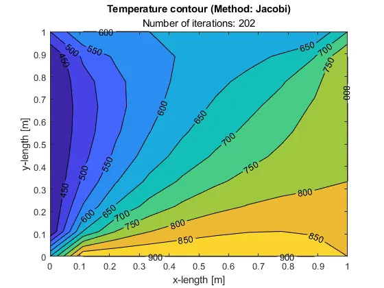
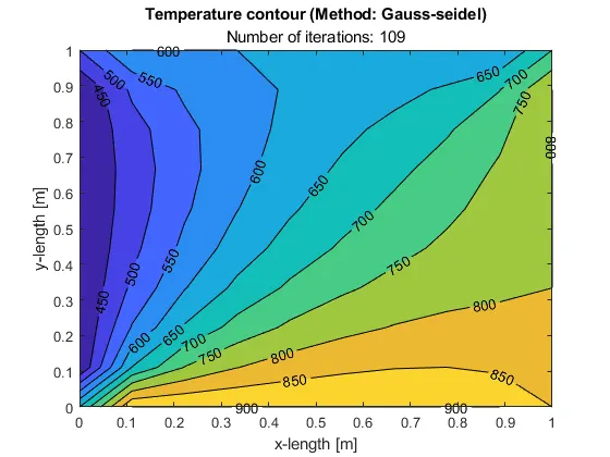
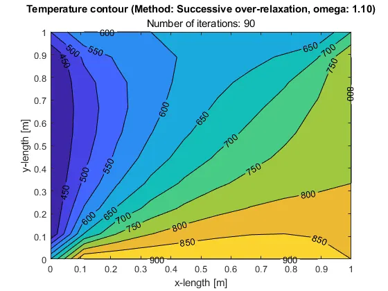
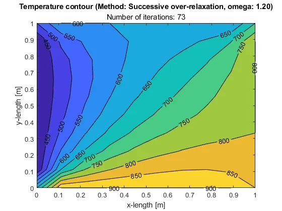
Final contour for all the methods show a similar Temperature profile. However the number of iterations required to attain this level of accuracy is different for different schemes. Gauss-seidel method takes about half the number of iterations to converge as compared to Jacobi. SOR method slightly improves upon Gauss-seidel method. Omega factor helps to speed up the convergence but it is to be kept in mind that over-relaxation could lead to instability due to over-shooting the solution.
2. Solve unsteady 2D heat conduction equation by using the point iterative techniques
`(delT)/(delt) = alpha((del^2T)/(delx^2) + (del^2T)/(dely^2))`
Discretizing the partial differential terms using truncated Taylor series - `n` represents the time-step number
`(delT)/(delx) = (T^(n+1) - T^n)/(Deltat)` -> Forward differencing
Using central differencing for spacial derivatives - `i` and `j` indices represent x and y node position respectively
`( del^2T)/(delx^2) = ( T_((i-1)(j)) - 2T_((i)(j)) + T_((i+1)(j)) ) / (Deltax)^2`
`( del^2T)/(dely^2) = ( T_((i)(j-1)) - 2T_((i)(j)) + T_((i)(j+1)) ) / (Deltay)^2`
If the T values on RHS of spacial derivative equations are taken from `n^(th)` time-step, the scheme is explicit. If it is from `(n+1)^(th)` time-step, the scheme is implicit.
2a. Explicit unsteady 2D heat conduction
Summing above euqations for partial derivatives in explicit formulation
`(T_((i)(j))^(n+1) - T_((i)(j))^n)/(Deltat) = alpha (( T_((i-1)(j))^n - 2T_((i)(j))^n + T_((i+1)(j))^n ) / (Deltax)^2 + ( T_((i)(j-1))^n - 2T_((i)(j))^n + T_((i)(j+1))^n ) / (Deltay)^2)`
Rearring for `T_((i)(j))^(n+1)`
`T_((i)(j))^(n+1) = T_((i)(j))^n + (alpha * Deltat)/ (Deltax)^2 ( T_((i-1)(j))^n - 2T_((i)(j))^n + T_((i+1)(j))^n ) + (alpha * Deltat)/ (Deltay)^2( T_((i)(j-1))^n - 2T_((i)(j))^n + T_((i)(j+1))^n )`
Taking `k1 = (alpha * Deltat)/ (Deltax)^2` and `k2 = (alpha * Deltat)/ (Deltay)^2`, above equ becomes
`T_((i)(j))^(n+1) = T_((i)(j))^n + k1 * ( T_((i-1)(j))^n - 2T_((i)(j))^n + T_((i+1)(j))^n ) + k2 *( T_((i)(j-1))^n - 2T_((i)(j))^n + T_((i)(j+1))^n )`
`T_((i)(j))^(n+1) = T_((i)(j))^n*(1 - 2k1 -2k2) + k1 * ( T_((i-1)(j))^n + T_((i+1)(j))^n ) + k2 *( T_((i)(j-1))^n + T_((i)(j+1))^n )`
For explicit scheme, CFL number = k1 + k2, should be less than or equal to 0.5 for a stable diffusion solution.
Discretize the domain similar to steady state analysis. Assume alpha = 1.4. Time-step size is chosen as 2e-3 based on CFL criteria. CFL number is close to but less than 0.5
Since all terms in RHS of the explicit scheme are known `T_((i)(j))^(n+1)` is directly calculated based on intial conditions and boundary conditions for different time-step.
Difference in temperature field between the time-steps is monitored and solution is stopped when the difference is less than the tolerance. i.e. steady state is reached
Matlab code:
% Solve unsteady 2D heat conduction equation
% by using the explicit techniques
% dT/dt = alpha * (d^2T/dx^2 + d^2T/dy^2)

%Taking `k1 = (alpha * Deltat)/ (Deltax)^2` ...
%   and `k2 = (alpha * Deltat)/ (Deltay)^2`, above equ becomes
% `T_((i)(j))^(n+1) = T_((i)(j))^n*(1 - 2k1 -2k2) ...
%       + k1 * ( T_((i-1)(j))^n + T_((i+1)(j))^n ) ...
%           + k2 *( T_((i)(j-1))^n + T_((i)(j+1))^n )`

clear all
close all
clc

% heat diffusion coefficient
alpha = 1.4;            % assumed value

% absolute error criteria
tolerance = 1e-4;

% Domain sizes
L_x = 1;        % Assume x length as 1 [m]
L_y = 1;        % Assume y length as 1 [m]
% Discretize domain (nx * ny)
nx = 10;        % number of nodes on x axis
ny = 10;        % number of nodes on y axis
% Node distances
Deltax = L_x/(nx-1);
Deltay = L_y/(ny-1);

% The Boundary conditions for the problem
% temperature in [K]
top_Boundary = 600;
bottom_Boundary = 900;
left_Boundary = 400;
right_Boundary = 800;
initial_temp = min([top_Boundary,bottom_Boundary,...
    left_Boundary,right_Boundary]);  % intial temperature for 1st iteration

% Initialize temperature in the domain
T = initial_temp*ones(ny,nx);

% Boundary conditions
T(1,:) = top_Boundary;
T(end,:) = bottom_Boundary;
T(:,1) = left_Boundary;
T(:,end) = right_Boundary;

% Set T at corners as mean of nearby nodes
T(1,1) = mean([T(1,2),T(2,1)]);
T(1,end) = mean([T(1,end-1),T(2,end)]);
T(end,1) = mean([T(end-1,1),T(end,2)]);
T(end,end) = mean([T(end-1,end),T(end,end-1)]);

% time-step size
Deltat = 2e-3;      % should be chosen so that CFL_no <= 0.5
max_ts = 1500;      % max number of time-steps to solved, if steady state is not achieved

% calculate constant 'k1' and 'k2' prior to iteration to save time
k1 = (alpha * Deltat)/ (Deltax)^2;
k2 = (alpha * Deltat)/ (Deltay)^2;
CFL_no = k1 + k2;

% variable to store the frames for unsteady temperature profile movie
M(max_ts) = struct('cdata',[],'colormap',[]);

% initialize error variable to a large value
diff = 1e9;

% solve the 2D heat conduction equation in explicit scheme
for ts = 1:max_ts
    T_old = T;      % T_old used to store temperature field at previous time-step
    for i = 2:nx-1
        for j = 2:ny-1

            % Calculate coefficients of discretized solution of T(i,j)
            term1_coeff = 1 - (2*k1) - (2*k2);

            % Calculate sum of neightboring Temperatures
            H = T(i-1,j) + T(i+1,j);
            V = T(i,j-1) + T(i,j+1);

            % Solve for T(i,j) using discretized equ
            T(i,j) = (term1_coeff * T_old(i,j)) + (k1 * H) + (k2 * V);
        end
    end

    % Create a domain using x and y variabled in space and
    % plot the contour of temperature on the grid
    x = linspace(0,L_x,nx);
    y = linspace(L_y,0,ny);
    contourf(x,y,T,'ShowText','on')
    titletext = sprintf("Time: %0.4f, Time-step: %d",ts*Deltat, ts);
    title("Temperature contour", titletext);
    xlabel("x-length [m]")
    ylabel("y-length [m]")
    pause(0.05)

    % capture frame for movie
    M(ts) = getframe(gcf);

    % max difference of Temperature between time-steps
    diff = max(abs(T - T_old),[],"all");
    % check if steady state is reached and break the time-loop
    if diff < tolerance
        break
    end
end

%Create movie until current time-step
M = M(1:ts);
movie(M)

% write movie using VideoWriter
videofile = VideoWriter('Temperature-explicit.avi','Uncompressed AVI');
open(videofile);
writeVideo(videofile,M);
close(videofile);
Results:
The solution reaches steady state fairly quickly in 130 time-steps. This is so since the domain is discretized with less number of points and alpha is taken a large value by assumption. In realty transient simulations usually take much longer to achieve steady-state compared to steady state solvers.
2b. Implicit unsteady 2D heat conduction
Summing discretized equations for partial derivatives in implicit formulation
`(T_((i)(j))^(n+1) - T_((i)(j))^n)/(Deltat) = alpha (( T_((i-1)(j))^(n+1) - 2T_((i)(j))^(n+1) + T_((i+1)(j))^(n+1) ) / (Deltax)^2 + ( T_((i)(j-1))^(n+1) - 2T_((i)(j))^(n+1) + T_((i)(j+1))^(n+1) ) / (Deltay)^2)`
Rearring for `T_((i)(j))^(n+1)` on LHS
`T_((i)(j))^(n+1) = T_((i)(j))^n + (alpha * Deltat)/ (Deltax)^2 ( T_((i-1)(j))^(n+1) - 2T_((i)(j))^(n+1) + T_((i+1)(j))^(n+1) ) + (alpha * Deltat)/ (Deltay)^2( T_((i)(j-1))^(n+1) - 2T_((i)(j))^(n+1) + T_((i)(j+1))^(n+1) )`
Taking `k1 = (alpha * Deltat)/ (Deltax)^2` and `k2 = (alpha * Deltat)/ (Deltay)^2`, above equ becomes
`T_((i)(j))^(n+1) = T_((i)(j))^n + k1 * ( T_((i-1)(j))^(n+1) - 2T_((i)(j))^(n+1) + T_((i+1)(j))^(n+1) ) + k2 *( T_((i)(j-1))^(n+1) - 2T_((i)(j))^(n+1) + T_((i)(j+1))^(n+1) )`
Taking `T_((i)(j))^(n+1)` on LHS
`T_((i)(j))^(n+1) + (k1* 2T_((i)(j))^(n+1)) + (k2* 2T_((i)(j))^(n+1)) = T_((i)(j))^n + k1 * ( T_((i-1)(j))^(n+1) + T_((i+1)(j))^(n+1) ) + k2 *( T_((i)(j-1))^(n+1) + T_((i)(j+1))^(n+1) )`
`T_((i)(j))^(n+1) * (1+2k1+2k2) = T_((i)(j))^n + k1 * ( T_((i-1)(j))^(n+1) + T_((i+1)(j))^(n+1) ) + k2 *( T_((i)(j-1))^(n+1) + T_((i)(j+1))^(n+1) )`
`T_((i)(j))^(n+1) = T_((i)(j))^n/(1+2k1+2k2) + ((k1)/(1+2k1+2k2)) * ( T_((i-1)(j))^(n+1) + T_((i+1)(j))^(n+1) ) + ((k2)/(1+2k1+2k2)) *( T_((i)(j-1))^(n+1) + T_((i)(j+1))^(n+1) )`
For implicit scheme, CFL number = k1 + k2, should not be a constraint to get a stable solution. However to get accurate solutions, a reasonably small value of CFL number has to be chosen.
Discretize the domain similar to steady state analysis. Assume alpha = 1.4. Time-step size is chosen as 1e-2 and CFL number is 2.2. For SOR scheme, solution is processed through time-step sizes of 1e-2 and 1e-1 corresponding to CFL number of 2.2 and 22.
Since all terms in RHS of the implicit scheme are not known, `T_((i)(j))^(n+1)` is to be calculated using an iterative method. Iterations are stopped when the error(max difference of Temperature between iterations) reach the specified value for a time-step. Difference in temperature field between the time-steps is monitored and solution is stopped when the difference(max difference of Temperature between time-steps) is less than the tolerance. i.e. steady state is reached. The following schemes are utilized for calculating the Temperature field within a time-step in iterative method.
The coefficients of RHS of discretized equation are solved first.
term1 = 1/(1+2k1+2k2) , term2 = k1 * term1, term3 = k2 * term1
Sum of horizontal neibhoring nodes are assigned to H and sum of vertical neighboring nodes are assinged to V
Finally the equation is solved as `T_((i)(j))^(n+1) = term1 * T^(n) + term2 * H + term3 * V`
Following methods are used to calculate H and V in above equation
1. Jacobi - H and V are calculated using values of T from previous iteration
2. Gauss-seidel - H and V are calculated using values of T from current iteration when available
3. Successive over-relaxation - T calculated from Gauss-seidel method is scaled using an over-relaxation factor
Matlab code:
% Solve unsteady 2D heat conduction equation
% by using the explicit techniques
% dT/dt = alpha * (d^2T/dx^2 + d^2T/dy^2)

% Taking `k1 = (alpha * Deltat)/ (Deltax)^2` ...
%   and `k2 = (alpha * Deltat)/ (Deltay)^2`, above equ becomes
% `T_((i)(j))^(n+1) = T_((i)(j))^n/(1+2k1+2k2) ...
%    + ((k1)/(1+2k1+2k2)) * ( T_((i-1)(j))^(n+1) + T_((i+1)(j))^(n+1) ) ...
%       + ((k2)/(1+2k1+2k2)) *( T_((i)(j-1))^(n+1) + T_((i)(j+1))^(n+1) )`

% Solve implicit equations using following methods
% 1. Jacobi
% 2. Gauss-seidel
% 3. Successive over-relaxation

clear all
close all
clc

% Choose from methods provided above to solve the 2D heat cond equ
method_names = ["Jacobi","Gauss-seidel","Successive over-relaxation"];
method = 3;
omega = 1.2;            % over-relaxation factor for sor scheme

% heat diffusion coefficient
alpha = 1.4;            % assumed value

% absolute error criteria
tolerance = 1e-4;

% Domain sizes
L_x = 1;        % Assume x length as 1 [m]
L_y = 1;        % Assume y length as 1 [m]
% Discretize domain (nx * ny)
nx = 10;        % number of nodes on x axis
ny = 10;        % number of nodes on y axis
% Node distances
Deltax = L_x/(nx-1);
Deltay = L_y/(ny-1);

% The Boundary conditions for the problem
% temperature in [K]
top_Boundary = 600;
bottom_Boundary = 900;
left_Boundary = 400;
right_Boundary = 800;
initial_temp = min([top_Boundary,bottom_Boundary,...
    left_Boundary,right_Boundary]);  % intial temperature for 1st iteration

% Initialize temperature in the domain
T = initial_temp*ones(ny,nx);

% Boundary conditions
T(1,:) = top_Boundary;
T(end,:) = bottom_Boundary;
T(:,1) = left_Boundary;
T(:,end) = right_Boundary;

% Set T at corners as mean of nearby nodes
T(1,1) = mean([T(1,2),T(2,1)]);
T(1,end) = mean([T(1,end-1),T(2,end)]);
T(end,1) = mean([T(end-1,1),T(end,2)]);
T(end,end) = mean([T(end-1,end),T(end,end-1)]);

% time-step size
Deltat = 1e-1;
max_ts = 1500;      % max number of time-steps to be solved, if steady state is not achieved

% calculate constant 'k1' and 'k2' prior to iteration to save time
k1 = (alpha * Deltat)/ (Deltax)^2;
k2 = (alpha * Deltat)/ (Deltay)^2;
CFL_no = k1 + k2;

% variable to store the frames for unsteady temperature profile movie
M(max_ts) = struct('cdata',[],'colormap',[]);

% initialize time-step diff variable to a large value
ts_diff = 1e9;

% intialize total_iter to keep track of total number of iterations
tot_iter = 0;

% solve the 2D heat conduction equation in explicit scheme
for ts = 1:max_ts
    T_prev_ts = T;      % T_prev_ts used to store temperature field at previous time-step
    iter = 0;           % iter used to track number of iteration per time-step
    error = 1e9;        % initialize error variable to a large value
    while error > tolerance
        T_old = T;      % T_old used to store temperature field at previous iteration
        for i = 2:nx-1
            for j = 2:ny-1

                % Calculate coefficients of discretized solution of T(i,j)
                term1 = 1/(1 + (2*k1) + (2*k2));
                term2 = k1 * term1;
                term3 = k2 * term1;

                % Calculate sum of neightboring Temperatures using Jacobi
                if method == 1
                    H = T_old(i-1,j) + T_old(i+1,j);
                    V = T_old(i,j-1) + T_old(i,j+1);

                % Calculate sum of neightboring Temperatures using Gauss_seidel
                else
                    H = T(i-1,j) + T(i+1,j);
                    V = T(i,j-1) + T(i,j+1);
                end

                % Solve for T(i,j) using discretized equ
                T(i,j) = (term1 * T_prev_ts(i,j)) + (term2 * H) + (term3 * V);

                 % Scale the Gauss_seidel temperature using omega factor
                 % for SOR method
                if method == 3
                    T(i,j) = ((1-omega) * T_old(i,j)) + (omega * T(i,j));
                end
            end
        end
        % calcualte iteration error
        error = max(abs(T - T_old),[],"all");
        % increment iteration count
        iter = iter + 1;
    end

    % add iter to total number of iterations
    tot_iter = tot_iter + iter;

    % Create a domain using x and y variabled in space and
    % plot the contour of temperature on the grid
    x = linspace(0,L_x,nx);
    y = linspace(L_y,0,ny);
    contourf(x,y,T,'ShowText','on')
    titletext1 = sprintf("%s (courant number: %0.4f)",method_names(method),CFL_no);
    titletext2 = sprintf("Time: %0.4f, Time-step: %d, Iter: %d, Total iter: %d",ts*Deltat, ts, iter, tot_iter);
    title("Temperature contour " + titletext1, titletext2);
    xlabel("x-length [m]")
    ylabel("y-length [m]")
    pause(0.05)

    % capture frame for movie
    M(ts) = getframe(gcf);

    % max difference of Temperature between time-steps
    ts_diff = max(abs(T - T_prev_ts),[],"all");
    % check if steady state is reached and break the time-loop
    if ts_diff < tolerance
        break
    end
end

%Create movie until current time-step
M = M(1:ts);
movie(M)

% write movie using VideoWriter
filename = sprintf("Temperature-implicit-%s-cfl-%.4f.avi",method_names(method),CFL_no);
videofile = VideoWriter(filename,'Uncompressed AVI');
open(videofile);
writeVideo(videofile,M);
close(videofile);
Based on the variable, method, the scheme used to solve the equation implicitly could be altered. omega is used to change the over-relaxation faction and Deltat is used to change the time-step size.
Results:
Jacobian method takes 57 time-steps to reach steady state with total number of iterations 1309
Gauss-seidel method also takes 57 time-steps to reach steady state with total number of iterations 815
SOR method also takes 57 time-steps to reach steady state with total number of iterations 561.
For a given `Deltat` the number of time-steps required to reach steady state is same with all the schemes. However the number of iterations used to converge the solution within each time-steps could be reduced by using Gauss-seidel or SOR schemes.
SOR method with courant number of 22 reaches steady state in 13 time-steps and total number of iterations 318.
With a larger `Deltat`steady state solution can be attained at a faster rate. However the number of iterations required to converge the solution within each time-step is larger with larger CFL number. Average number of iterations per time-step is around 20 for CFL number of 22, where it was around 10 for CFL number of 2.2.
The total time taken to reach the steady state is 1.3s (13 * `Deltat`) with CFL number 22 simulation. For simulations with courant number of 2.2, steady state was reached at 0.57s. Hence with larger time-steps, time-accurate solutions will be difficult to obtain. The important timelines could be overshot. To get time-accurate solutions at each time-step, small courant numbers are preferred even though implicit solutions are stable at larger values of courant number. To get a steady solution from unsteady approach and disregard the time-parameter, a larger CFL number approach could be used. The final Temperature field is same with either of the CFL options and different iteration schemes.