Week 3.5 - Deriving 4th order approximation of a 2nd order derivative using Taylor Table method

Aim: To derive the 4^th order approximations scheme of second order derivative for

1. Central difference
2. Skewed right sided difference
3. Skewed left sided difference

prove that your skewed schemes are fourth order accurate.

Deriving the 4^th order scheme of the second order derivative:

• Central Difference:

To compute fourth order central difference approximation of second order derivative at a point x we need 4 extra point with the current point i.e., two on the left and two on right side.

Now, we are considering the hypothesis equation as,

`(∂^2 f)/(∂x^2 )=af(x-2dx)+bf(x-dx)+cf(x)+df(x+dx)+ef(x+2dx) A)`

Then calculate the values of a, b, c, d, e then you get the required approximation. These values can be found out by using taylor ‘s table.

	`f(x)`	`f^' (x)dx`	`(f"(x)dx^2)/2!`	`(f^iii (x)dx^3)/3!`	`(f^iv (x)dx^4)/4!`	`(f^v (x)dx^5)/5!`	`(f^vi (x)dx^6)/6!`
`a*f(x-2*dx)`	a	-2a	4a	-8a	16a	-32a	64a
`b*f(x-dx)`	b	-b	b	-b	b	-b	b
`c*f(x)`	c	0	0	0	0	0	0
`d*f(x+dx)`	d	d	d	d	d	d	d
`e*f(x+2*dx)`	e	2e	4e	8e	16e	32e	64e
`∑_(rows )▒〖=(∂^2 f)/(∂x^2 )〗`	0	0	1	0	0	?	?

Since we are trying to calculate 2^nd order derivative the only term, we need to consider on RHS is second order derivative. So, we can assign 1 to that 2^nd order derivative.

Now formulating the above equation, we will have,

`a+b+c+d+e=0 (1) -2a-b+0+d+2e=0 (2) 4a+b+0+d+4e=2 (3) -8a-b-0+d+8e=0 (4) 16a+b+0+d+16e=0 (5)`

Now writing this above equation in AX = b in MATLAB We will have,

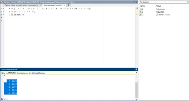
So, from above equation A),

`(∂^2 f)/(∂x^2 )=-0.0833f(x-2dx)+1.3333f(x-dx)-2.5000f(x)+1.3333f(x+dx)-0.0833f(x+2dx) (B)`

To show derived that derived Central scheme is of 4^th order approximation we should use following given below formula:

The order of accuracy (P) = No. of nodes in stencil(N) – order of derivative(Q) +1

P = 5 – 2 + 1 = 4

Hence order of derived scheme is of the 4^th order.

• Skewed Right sided difference:

To compute fourth order skewed right difference approximation of second order derivative at a point x we need 5 extra point with the current point i.e., and 6 on right side.

Now, we are considering the hypothesis equation as,

`(∂^2 f)/(∂x^2 )=af(x)+bf(x+dx)+cf(x+2dx)+df(x+3dx)+ef(x+4dx)+g(x+5dx) C)`

Then calculate the values of a, b, c, d, e then you get the required approximation. These values can be found out by using taylor ‘s table.

	`f(x)`	`f^' (x)dx`	`(f"(x)dx^2)/2!`	`(f^iii (x)dx^3)/3!`	`(f^iv (x)dx^4)/4!`	`(f^v (x)dx^5)/5!`	`(f^vi (x)dx^6)/6!`
`a*f(x)`	a	0	0	0	0	0	0
`b*f(x+dx)`	b	b	b	b	b	b	b
`c*f(x+2*dx)`	c	2c	4c	8c	16c	32c	64c
`d*f(x+3*dx)`	d	3d	9d	27d	81d	243d	729d
`e*f(x+4*dx)`	e	4e	16e	64e	256e	1024e	4096e
`g(x+5dx)`	g	5g	25g	125g	625g	3125g	15625g
`∑_(rows )▒〖=(∂^2 f)/(∂x^2 )〗`	0	0	1	0	0	?	?

Since we are trying to calculate 2^nd order derivative the only term, we need to consider on RHS is second order derivative. So, we can assign 1 to that 2^nd order derivative.

Now formulating the above equation, we will have,

`a+b+c+d+e+g=0 (1) b+2c+3d+4e+5g=0 (2) b+4c+9d+16e+25g=2 (3) b+8c+27d+64e+125g=0 (4) b+16c+81d+256e+625g=0 (5) b+32c+243d+1024e+3125g=0 (6)`

Now writing this above equation in AX = b in MATLAB We will have, values of a to g,

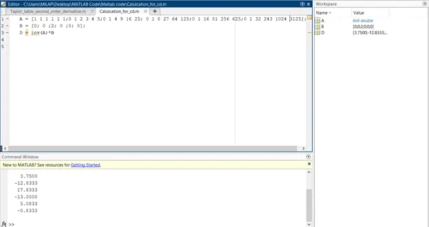
a = 3.7500

b = -12.8333

c = 17.8333

d = -13.0000

e = 5.0833

f = -0.8333

So, from above equation C),

`(∂^2 f)/(∂x^2 )=3.75f(x)-12.8333f(x+dx)+17.8333f(x+2dx)-13f(x+3dx) 5.0833f(x+4dx)-0.8333f(x+5dx) (D)`

To show that derived skewed scheme is of 4^th order approximation we should use following given below formula:

The order of accuracy (P) = No. of nodes in stencil(N) – order of derivative(Q)

P = 6– 2 = 4

Hence order of derived scheme is of the 4^th order.

• Skewed Left sided difference:

  To compute fourth order skewed left difference approximation of second order derivative at a point x we need 5 extra point with the current point i.e., and 6 on left side.

`(∂^2 f)/(∂x^2 )=af(x)+bf(x-dx)+cf(x-2dx)+df(x-3dx)+ef(x-4dx)+g(x-5dx) E))`

Then calculate the values of a, b, c, d, e then you get the required approximation. These values can be found out by using taylor ‘s table.

	`f(x)`	`f^' (x)dx`	`(f"(x)dx^2)/2!`	`(f^iii (x)dx^3)/3!`	`(f^iv (x)dx^4)/4!`	`(f^v (x)dx^5)/5!`	`(f^vi (x)dx^6)/6!`
`a*f(x)`	a	0	0	0	0	0	0
`b*f(x-dx)`	b	-b	b	-b	b	-b	b
`c*f(x-2*dx)`	c	-2c	4c	-8c	16c	-32c	64c
`d*f(x-3*dx)`	d	-3d	9d	-27d	81d	-243d	729d
`e*f(x-4*dx)`	e	-4e	16e	-64e	256e	-1024e	4096e
`g(x-5dx)`	g	-5g	25g	-125g	625g	-3125g	15625g
`∑_(rows )▒〖=(∂^2 f)/(∂x^2 )〗`	0	0	1	0	0	?	?

Since we are trying to calculate 2^nd order derivative the only term, we need to consider on RHS is second order derivative. So, we can assign 1 to that 2^nd order derivative.

Now formulating the above equation, we will have,

`a+b+c+d+e+g=0 (1) -b-2c-3d-4e-5g=0 (2) b+4c+9d+16e+25g=2 (3) -b-8c-27d-64e-125g=0 (4) b+16c+81d+256e+625g=0 (5) -b-32c-243d-1024e-3125g=0 (6)`

Now writing this above equation in AX = b in MATLAB We will have, values of a to g,

a = 3.7500

b = -12.8333

c = 17.8333

d = -13.0000

e = 5.0833

f = -0.8333

So, from above equation C),

`(∂^2 f)/(∂x^2 )=3.75f(x)-12.8333f(x-dx)+17.8333f(x-2dx)-13f(x-3dx) 5.0833f(x-4dx)-0.8333f(x-5dx) (D)`

To show that derived skewed scheme is of 4^th order approximation we should use following given below formula:

The order of accuracy (P) = No. of nodes in stencil(N) – order of derivative(Q)

P = 6– 2 = 4

Hence order of derived scheme is of the 4^th order.

Code for showing comparison of error in above Given schemes.

clear all
close all
clc 

%Define the function 
f= (@(x) exp(x)*cos(x));

% Calculation of the coefficients of central differencing difference scheme
a1=[1 1 1 1 1;-2 -1 0 1 2;4/2 1/2 0 1/2 4/2;-8/6 -1/6 0 1/6 8/6;16/24 1/24 0 1/24 16/24;];
c1=[0;0;1;0;0;];
xc=zeros(5,1);
xc=(a1^-1)*c1;

a2=[1 1 1 1 1 1;0 1 2 3 4 5;0 1/2 4/2 9/2 16/2 25/2;0 1/6 8/6 27/6 64/6 125/6;0 1/24 16/24 81/24 256/24 625/24;0 1/120 32/120 243/120 1024/120 3125/120;];
c2=[0;0;1;0;0;0;];
xr=zeros(6,1);
xr=(a2^-1)*c2;


%Assuming the value of x 
x = pi/3;
%Range of dx (grid spacing)
dx = linspace(pi/10,pi/100,10);

%Analytical derivative of function exp(x)*cos(x)

Analytical_derivative = -2*exp(x)*sin(x);

%Computing 4th order approximation of different schemes of the 2nd order derivative for given function 
for i = 1:length(dx)
    Central_difference(i) =((xc(1))*f(x-2*dx(i))+(xc(2))*f(x-dx(i))+(xc(3))*f(x)+(xc(4))*f(x+dx(i))+(xc(5))*f(x+2*dx(i)))/(dx(i))^2;
    Skewed_right_side_difference(i) =  ((xr(1))*f(x)+(xr(2))*f(x+dx(i))+(xr(3))*f(x+2*dx(i))+(xr(4))*f(x+3*dx(i)) +(xr(5))*f(x+4*dx(i))+(xr(6)*f(x+5*dx(i))))/(dx(i))^2;
    Skewed_left_side_difference(i) = ((xr(1)*f(x)+(xr(2))*f(x-dx(i))+(xr(3))*f(x-2*dx(i))+(xr(4))*f(x-3*dx(i))+(xr(5))*f(x-4*dx(i))+(xr(6))*f(x-5*dx(i))))/(dx(i))^2;
    %Calculate the absolute error 
   Central_difference_error(i)= abs(Analytical_derivative - Central_difference(i));
   Skewed_right_side_difference_error(i) = abs(Analytical_derivative - Skewed_right_side_difference(i));
   Skewed_left_side_difference_error(i) = abs(Analytical_derivative -Skewed_left_side_difference(i));
end 

%Plotting graph dx vs value of error for derived fourth order schemes 
loglog(dx,Central_difference_error)
hold on
loglog(dx,Skewed_right_side_difference_error)
hold on
loglog(dx,Skewed_left_side_difference_error)
title('Change of error as factor of dx for different 4th order schemes for given function x = pi')
xlabel('dx(grid size)')
ylabel('value of error')
legend('Central Difference Error','Skewed Right side Difference Error','Skewed Left side Difference Error')

Explaination:

• Here in this code first function given in problem is defined in the code.
• Later values of x and dx, and coefficient for central differencing schemes and skewed schemes was defined.
• To compare the result with actual result analytical derivative is also calculated in the code.
• here we have to use range of dx value so that for loop is introduced in CODE.
• also various schemes which was discussed above is implemented in the code.
• By comparing with analytical result absolute error is also calculated and plotted.
• Here to plot loglog function is used and hold command is used to combine plotting of all three results.

Plot:

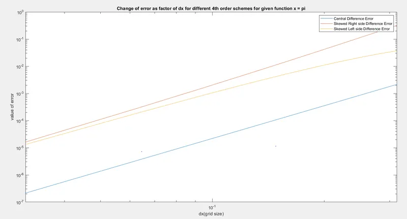
From the above plot we can conclude that how error is varying with respect to values of dx. The error is decreasing as the grid size is decreasing and also central differencing scheme is more accurate than skewed right side and skewed left side scheme. The higher order of scheme is the lower the error is going to be for same grid size. But in actual when the geometry is very complex and when the flow become very complex, we can not always use higher order method and in order to use for simulation to run commercial codes one should always go to first order scheme for getting solution.

Importance of skewed scheme:

When we want to calculate the value of function at the boundary, we cannot use central difference schemes because it requires the value of nodes on both the sides, whereas in skewed scheme we can use value of only one side.

This is where skewed scheme come to in picture, it is uniqueness of skewed scheme which central difference scheme cannot do, but in terms of accuracy central differencing scheme is more accurate.