Linear Convection for varying timesteps

Aim: To write a code in MATLAB for the Numerical solution for one dimensional equation by varying Timesteps

Objectives:

• To solve the 1D Linear convection equation
• The solution is to be calculated using different no. of timesteps
• Taking initial velocities constant, final velocity is compared across different time steps.

One dimensional linear convection equation:

The equation under the focus is,

`∂u/∂t + c*∂u/∂x =0`

Above equation will be solved using time marching procedure, i.e., velocities will be solved at each node for each timestep and it will be done to all predefined steps.

The initial condition is predefined at timestep and it is used to compute velocity profiles for next iteration. Similarly other timesteps are calculated using previous condition timesteps.

The velocity at node2 for 2^nd timestep is calculated as below.

`∂u/∂t + c*〖∂u/∂x|〗_2`

`(u_2^2-u_(2 )^1)/(∆t )+c((u_2^1-u_1^1)/∆x)=0`

`u_2^2=u_2^1-c*∆t/∆x[u_2^1-u_1^1]`

Similarly, the velocity at node 3,

`(u_2^3-u_(2 )^2)/(∆t )+c((u_2^2-u_1^2)/∆x)=0`

`u_2^3=u_2^2-c*∆t/∆x[u_2^2-u_1^2]`

In general, it can be written as,

`(u_2^(n+1)-u_(2 )^n)/(∆t )+c((u_2^n-u_1^n)/∆x)=0`

`u_2^(n+1)=u_2^n-c*∆t/∆x[u_2^n-u_1^n]`

Similarly, we can calculate for the velocities at all nodes for further. Generalized equation for it is given below.

`∂u/∂t+c ∂u/∂x |_T`

`(u_T^(n+1)-u_(T )^n)/(∆t )+c((u_T^n-u_T^n)/∆x)=0`

`u_T^(n+1)=u_T^n-c*∆t/∆x[u_T^n-u_T^n]`

MATLAB program to implement the above explained method to solve for 1D Convection equation.

The initial condition for code is given below.

1. Domain length = 1m
2. The initial velocity profile is step function where velocity is 2m/s between x = 0.1 & 0.3 and 1 m/s everywhere else.

Other Important details are given below.

1. Constant convection coefficient (C) = 1 m/s
2. Time steps are varied = [1e-4 1e-3 1e-2 1e-1]
3. Simulation run time = 0.4 second
4. The no. of node is taken 81 for the s

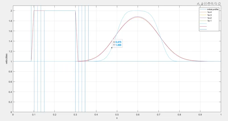
In Problem is 4 different nodes value is given. The MATLAB Code to entertain such data is given below, along with the plot. In this all the four time steps plotted together. From the plots it can be seen that lesser the value of time step better the convergence.

%Solution for Varying time steps for 1D Convection eqn  %
clear all 
close all 
clc 

% Assigining initial values%
L = 1; % Length of Domain  
n = 81; %No. of  nodes 
c = 1; % Constant 
t = 0.4; % Simulation time 
dt = [1e-4 1e-3 1e-2 1e-1]; % Time steps arrays
x = linspace(0,L,n); % Total no. of interval in domain length 
dx = L/(n-1); % (grid size)

%Loop for different values of time steps 

for j = 1:length(dt)
    nt(j) = t/dt(j);
    %To get value of velocity 2m/s in b/w 0.1 to 0.3 seconds we can define
    %n_start & n_end 
    
    n_start = 9;
    n_end   = 25;
    
    %Lines to assign values of velocities to nodes% 
    
    u = 1*ones(1,n);
    u(n_start:n_end) = 2;
    %Below line will update initial value for future updation %
    
    u_old = u;
    u_initial = u;
    
    %loop starts for time step integration 
    for i = 1:nt(j)
        
        %loop to calculate the velocity at each node at a given time step 
        for k = 2:(n-1) 
            u(k) = u_old(k) -(c*dt(j)/dx)*(u_old(k)-u_old(k-1));
        end 
        
        %To take the refferance value of next time step update the velocity
        u_old = u; 
    end 
    
    %Below lines will be used to plot the lines the velocity profile at
    %given time step %
    
    figure(1)
    plot(x, u_initial);
    
    hold on;
    
    plot(x,u);
    axis([0 1 0 2.1]);
    
    grid on; 
    xlabel('x');
    ylabel('velocities');
    legend(dt);
    hold on ; 
end 
legend('initial profile','1e-4','1e-3','1e-2','1e-1');