Linear Convection for varying number of nodes

Aim: To write a code in MATLAB for the Numerical solution for one dimensional equation by varying number of nodes

Objectives:

1)To solve the 1D Linear convection `∂u/(∂t )+c*∂u/∂x=0`

2)The solution is to be calculated using different no. of nodes

3)Taking initial velocities constant, final velocity is compared across all set of the nodes.

One dimensional linear convection equation:

The equation under the focus is,

`∂u/∂t+c*∂u/∂x =0`

Above equation will be solved using time marching procedure, i.e., velocities will be solved at each node for each timestep and it will be done to all predefined steps.

The initial condition is predefined at timestep and it is used to compute velocity profiles for next iteration. Similarly other timesteps are calculated using previous condition timesteps.

The velocity at node2 for 2^nd timestep is calculated as below.

`∂u/∂t+c*〖∂u/∂x|〗_2`

`(u_2^2-u_(2 )^1)/(∆t )+c((u_2^1-u_1^1)/∆x)=0`

`u_2^2=u_2^1-c*∆t/∆x[u_2^1-u_1^1]`

Similarly, the velocity at node 3,

`(u_2^3-u_(2 )^2)/(∆t )+c((u_2^2-u_1^2)/∆x)=0`

`u_2^3=u_2^2-c*∆t/∆x[u_2^2-u_1^2]`

In general, it can be written as,

`(u_2^(n+1)-u_(2 )^n)/(∆t )+c((u_2^n-u_1^n)/∆x)=0`

`u_2^(n+1)=u_2^n-c*∆t/∆x[u_2^n-u_1^n]`

Similarly, we can calculate for the velocities at all nodes for further. Generalized equation for it is given below.

`∂u/∂t+c ∂u/∂x |_T`

`(u_T^(n+1)-u_(T )^n)/(∆t )+c((u_T^n-u_T^n)/∆x)=0`

`u_T^(n+1)=u_T^n-c*∆t/∆x[u_T^n-u_T^n]`

MATLAB program to implement the above explained method to solve for 1D Convection equation.

The initial condition for code is given below.

1. Domain length = 1m
2. The initial velocity profile is step function where velocity is 2m/s between x = 0.1 & 0.3 and 1 m/s everywhere else.

Other Important details are given below.

1. Constant convection coefficient (C) = 1 m/s
2. Time steps dt = 0.01 second
3. Simulation run time = 0.4 second

In Problem is 4 different nodes value is given. The MATLAB Code to entertain such data is given below.

%Matlab program to perform for different no of nodes in linear convection %
%Clearing command%
clear all
close all
clc 

%Assigning initial value% 
L = 1;
n = [20 40 80 160];
c = 1;
t = 0.4;
dt = 1e-2;
nt = t/dt;

%Calulation%
[q, u, dx] = linear_convection_fun(n,L);
u_initial = u;

for k = 1:length(n)
    figure(k)
    v = u{1,k};
    cf1 = (c*dt)/dx(k);
    %For loop for number of time steps 
    for i = 1:nt
        %for loop for all grid velocities values in mesh% 
        for j = 2:length(q{1,k})
            z(j) = v(1,j)-(c*dt)/dx(k)*(v(1,j)-v(1,j-1));
        end
        z(1) = 1;
        v = z;
        plot(q{1,k},u{1,k},'color','y','linewidth',3)
        hold on 
        plot(q{1,k},z,'r')
        pause(0.3)
        axis([0 1 0 2])
    end 
    hold off 
end
            

%Loop for different number of nodes %
for i = 1:length(n)
    
    %Defining x and dx for different values for number of nodes %
    x = linspace(0, L,n(i));
    dx = x(2)-x(1);
    
    %Eqaution to use get the node numbers for step profile for velocity in
    %initial time step
   n_start(i) = [3 5 9 17];
   n_end(i) = [ 7 13 25 49];
   
end
%Below lines are used to assign the initial condition 
u = 1*ones (1,n(i));
u(n_start(i):n_end(i)) = 2;

%Below lines are update the initial velocity for future update and
%refference 
u_old = u;
u_initial = u;

%loop start for the time step integration 
for j = 1:nt 
    
    % loop to calculate the velocity at each node at a given time step 
    for k = 2:n(i)
        u(i) = u_old(i)- (c*dt/dx)*(u_old(i)-u_old(i-1));
    end 
    
   %update the value of velocity for next refference point %
   u_old = u;
   
   %Following set of lines is used to plot the velocity profile at given
   %time step 
   figure(fig)
   
   subplot(1,2,1);
   plot(x,u_initial, 'color','b');
   grid on; 
   axis([0 1 0 2.1]);
   xlabel('x');
   ylabel('Velocity');
   
   pause(0.1);
end 

fig = fig + 1;

Description of code:

1. Used clear commands to clear the data in present interface.
2. Assigned the required variables.
3. Used function command ‘linear_convection_fun’ to get the data to plot the intial velocity profile for given different no. of nodes profiles.
4. Used different loop which was mentioned on code itself to calulate velocity data and plot the result of simulation time itself by using ‘pause’ command.
5. Axis command have used to sex axis bound.
6. ‘hold on’ command used so that It wouldn’t clear the axis properties for future plots.

Function code:

%Find start & stop value, U Values%
function [ q, v, dx] = linear_convection_fun(n,L)

for i = 1:length(n)
    q{1,i} = linspace(0,L,n(i)); %Mesh generation
    x = q{1,i};
    dx(i) = x(2) -x(1);          %Grid spacing 
    u = 1*ones(1,n(i));          %Intial velocities 
    A = logical(x>=0.1 & x<=0.3);
    index = find(A==1);
    n_start = index(1);
    n_end   = index(end);
    u(n_start:n_end) = 2;
    v{1,i} = u;
end
end

Description of function code:

1. Here used function code to find mesh discretization, grid spacing, velocities profile data, start and end points for grid location. (0.1 & 0.3 m)
2. Using different logical operators u = 2m/s has assigned. Apart from other location velocity u = 1 m/s has assigned.

Numerical diffusion:

It would be arising because of truncation has been used. It basically a combination of dispersion and dissipation.

Courant number:

This number will enable us to check stability of model w.r.t grid spacing and time step.

`Courant number(C_0 )=c∆t/∆x`

1. If = 1, then local truncation error is zero, hence no Numerical diffusion.
2. If > 1, then local truncation error is -ve, hence its causes of instability.
3. If ><1 then local truncation error is +ve, hence its causes Numerical diffusion effect. 1) No. of nodes = 20

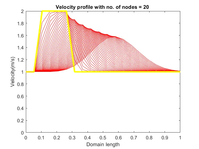
Results: `C_0=0.19 (<1),Hence diffusion occrus.`

2) No. of nodes = 40

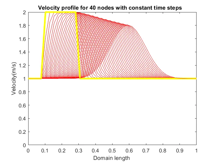
Result: `C_0=0.39(<1).Hence diffusion occurs.`

3) No. of nodes = 80

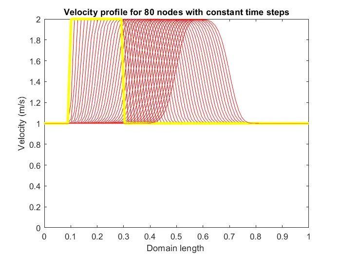
`Result: `C_0=0.79 (<1),Hence diffusion occurs.`

4)No. of nodes

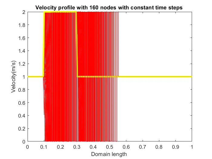
Result: `C_0=1.59>1 ,so it becomes unstable.`

Conclusions:

1. From the above set of plots, it can be seen that initial velocity profile accuracy will improve as the number of nodes increases.
2. With increase in number of nodes artificial diffusion is reduced. Although in 4^th plot solution become unstable.