Week 7 - Simulation of a 1D Super-sonic nozzle flow simulation using Macormack Method
Project Abstract:
This project presents modelling of behaviour of fluid and its properties when it passes through a convergent divergent nozzle by Macormack method. However to simplyfy it only 1D flow is considered in which flow is varied in x axis only. MATLAB code is used to understand the governing eqaution of the flow is transformed into Numeric form(Finite Difference form). Macormack predictor corrector explicit finite difference method is used as solver. The flow type is ''Qussi 1Dincompressible unsteady inviscid isentropic flow".
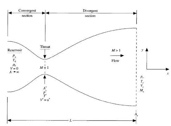
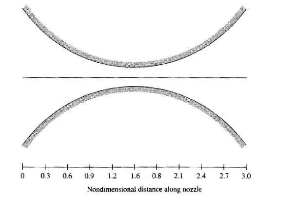
Here the steady isentropic flow through convergent divergent nozzle is considered. The flow details at the inlet and outlet are denoted in the figure shown along with the coordinate of the nozzle. As we are assuming that the flow of properties will be varied in only X direction therfore this flow will become 1D Flow.
The governing eqaution for one dimensional flow nozzle will be expressed as following.
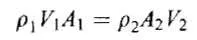
Continuity eqaution will be written by,
Momentum eqaution will be written by,

Same way energy eqaution is written by,
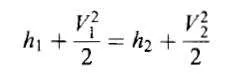
Here 1 & 2 denotes the quantity at different location of the nozzle.
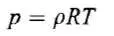
further perfect gas eqaution is written by,
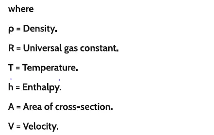
now let us consider the non conservative form of governing eqaution.
Initial condition and nozzle shape:
Nozzle is kept constant at time. The parabolic area is expressed by following eqaution.

At x = 1.5 m is the throat of nozzle. The convergent region is at region in between [0,1.5] whereas divergent section occupies the region in between [1.5,3].
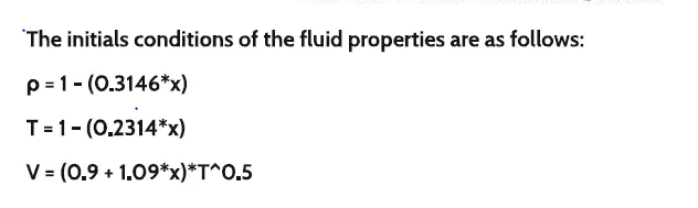
The initial conditions for fluid properties are given below.
Boundary Conditions:
The subsonic flow condition: Here velocity to float was chosen because on a physical basis we know mass flow through nozzle must be allowed to adjust to proper steady state and allowing proper V to float make the sense with adjustment.
The independent parameters ,
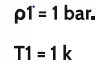
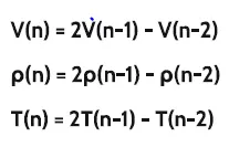
The values of Velocity density and temperature can be expressed by following way based on linear extrapolation.
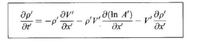
Nondimensional non conservative form of above governing eqaution are ,
Continuity eqaution,
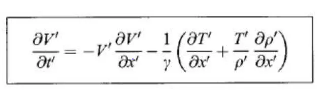
Momentum eqaution,
Energy eqaution,

Here in above three eqautions prime variables indicates the nondimensional form.The above eqaution is nonconservative in nature. Here maccormack predictor corrector explicit method will be to determine the depedent variables.
In predictor method forward difference scheme of 1st order is used to determine the variable for next iteration. While in corrector method backward difference scheme of 1st order is used to determine the variable for next iteration.
Discretization of the PDE using Maccormack explicitily method.
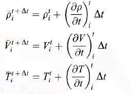
Predictor step (1st Order forward difference scheme):



The predicted value of `rho, V, t` for the next time step will be,
Corrector step(1st Order backward differrence scheme)
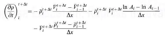

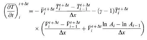
The average time derivative for all the premitive variables are
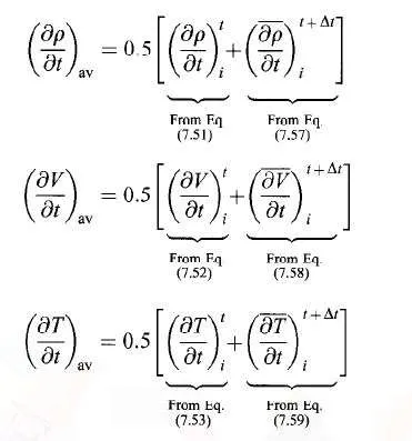
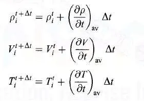
therefore the corrected values for flowfield is t+dt are given below,
Nondimensinalised Conservation form of governing eqaution :
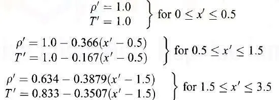
Initial Conditions,
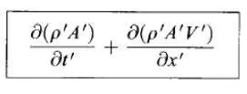
Continuity eqaution,
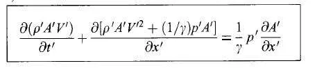
Momentum eqaution,
Energy eqaution,

The above eqaution are nondimensionalise conservative form of mass,momentum and energy eqaution.
It can be expressed in generic form by follwing way.
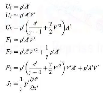
Therefore the above governing eqaution can be written as,
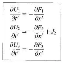
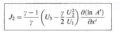
Before directly discretizing the above generic form we must express the premitive values in terms of the solution vector has to be converted into the flux terms.
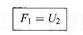
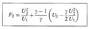
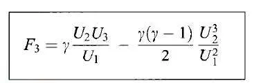
Coding part:
Main code for nozzle:
%% Main script for 1D Supersonic nozzle flow%%
clear all
close all
clc

%%1D Grid Generation%%
n = 61;
x = linspace(0,3,n);
dx = x(2)-x(1);
A = 1+2.2*(x-1.5).^2;
gamma = 1.4;
c = 0.5;   % CFL No.
n_throat = find(A-1<0.001);

%% Conservative %%
[rho_c,V_c,T_c,P_c,mass_flow_c,Mach_c,rho_throat,T_throat,Mach_throat,P_throat] = Conservative_code(n,x,dx,A,gamma,n_throat,c)
% fprintf('Min no of iteration to convergence for conservation form:%fn',iter)

%Steady properties of nozzle %%
figure(3)
subplot(4,1,1)
plot(x,rho_c,'g','linewidth',1)
title('Steady state properties at nozzle(Conservative form)')
xlabel('x/L')
ylabel('rho/rho_0')
legend('Density ratio')

subplot(4,1,2)
plot(x,T_c,'b','linewidth',1)
xlabel('x/L')
ylabel('Temperature ratio')
legend('Temperature ratio')

subplot(4,1,3)
plot(x,P_c,'y','linewidth',1)
xlabel('x/L')
ylabel('Pressure ratio')
legend('Pressure ratio')


subplot(4,1,4);
plot(x,Mach_c,'r','linewidth',1)
xlabel('x/L')
ylabel('Mach No.')
legend('Mach ')

% subplot(4,1,5)
% plot(x,V_c,'O','linewidth',1)
% xlabel('x/L')
% ylabel('Velocity.')
% legend('Velocity ')

%%Transient properties at the throat of nozzle %%
figure(4)
subplot(4,1,1)
plot(rho_throat)
title('Transient properties variation at the nozzle throat(Conservative form')
xlabel('Time steps')
ylabel('Density')
grid on

subplot(4,1,2)
plot(P_throat)
xlabel('Time steps')
ylabel('Pressure')
grid on

subplot(4,1,3)
plot(T_throat)
xlabel('Time steps')
ylabel('Temperature')
grid on

subplot(4,1,4)
plot(Mach_throat)
xlabel('Time steps')
ylabel('Mach No.')
grid on


% subplot(4,1,5)
% plot(Velocity)
% xlabel('Time steps')
% ylabel('Velocity')
% grid on

% %% Non- Conservative %%
[rho,V,T,P,mass_flow,Mach,rho_throat,T_throat,Mach_throat,P_throat] = non_conservative(n,x,dx,A,gamma,n_throat,c);
% fprintf('Min no of iteration to convergence for conservation form:%fn',iter);

%%Steady properties of nozzle%%
figure(5)
subplot(4,1,1)
plot(x,rho,'g','Linewidth',1)
title('Steady state properties at nozzle (Non conservative form)')
xlabel('x/L')
ylabel('rho/(rho_0)')
legend('Density ratio')
grid minor;

subplot(4,1,2)
plot(x,T,'b','Linewidth',1)
title('Steady state properties at nozzle (Non conservative form)')
xlabel('x/L')
ylabel('Temperature ratio')
legend('Temperature ratio')
grid minor

subplot(4,1,3);
plot(x,P,'y','Linewidth',1)
title('Steady state properties at nozzle (Non conservative form)')
xlabel('x/L')
ylabel('Pressure ratio')
legend('Pressure ratio')
grid minor

subplot(4,1,4)
plot(x,Mach,'r','Linewidth',1)
title('Steady state properties at nozzle (Non conservative form)')
xlabel('x/L')
ylabel('Mach No')
legend('Mach No')
grid minor

%%Transient properties at the throat of nozzle

figure(6)
subplot(4,1,1)
plot(rho_throat)
title('Transient properties variation at the nozzle throat(Non Conservative)')
xlabel('Time steps')
ylabel('Density')
grid on

subplot(4,1,2);
plot(P_throat);
xlabel('Time steps')
ylabel('Pressure')
grid on;

subplot(4,1,3)
plot(T_throat)
xlabel('Time steps')
ylabel('Temperature')
grid on;

subplot(4,1,4)
plot(Mach_throat)
xlabel('Time steps')
ylabel('Mach No')
grid on

figure(7)
plot(x,mass_flow_c)
hold on
plot(x,mass_flow)
xlabel('Length of nozzle')
ylabel('Mass flow rate')
legend('Conservative Mass flow rate','Non conservative mass flow rate')
Function code for Conservation form:
%%Conservative form approach%%
function[rho_c,V_c,T_c,P_c,mass_flow_c,Mach_c,rho_throat,T_throat,Mach_throat,P_throat] = Conservative_code(n,x,dx,A,gamma,n_throat,c)

%%Ininitial condition%%
for i = 1:length(x)
    if x(i)>= 0 && x(i)<= 0.5
        rho_c(i) = 1;
        T_c(i) = 1;
    end
    if x(i)>= 0.5 && x(i)<= 1.5
        rho_c(i) = 1 - 0.366*(x(i) - 0.5);
        T_c(i) = 1 - .167*(x(i) -0.5);
    end
    if x(i)>= 1.5 && x(i)<= 3.5
        rho_c(i) = 0.634- 0.3879*(x(i)-1.5);
        T_c(i) = 0.833- 0.3507*(x(i)-1.5);
    end
end
V_c = 0.59./(rho_c.*A);   % Velocity%
P_c = rho_c.*T_c;           % Pressure%

%Initial condition for the solution vectors
U_1 = rho_c.*A;
U_2 = (rho_c.*V_c).*A;
U_3 = rho_c.*A.*(((T_c./(gamma-1)+ (gamma/2)*(V_c.^2))));


nt =1400;
% iter = 0;
for k = 1:nt
    %     iter = iter+1;

    U_1_old = U_1;
    U_2_old = U_2;
    U_3_old = U_3;

    F_1 = U_2;
    F_2 = ((U_2.^2)./U_1) + (((gamma-1)/gamma)*(U_3 - ((gamma/2)*(U_2.^2./U_1))));
    F_3 = (gamma*(U_2.*U_3)./U_1)-((gamma*(gamma-1)/2).*((U_2.^3)./U_1.^2));

    %Defining the timeloop using cfl no
    a = sqrt(T_c);
    timestep = c*dx./(a+V_c);
    dt = min(timestep);

    %Initialising the predictor step
    for j = 2:n-1

        %Source vector
        J_2(j) = (1/gamma)*rho_c(j)*T_c(j)*((A(j+1)-A(j))/dx);

        %Continuity eqaution
        dU1_dt_p(j) = -((F_1(j+1)-F_1(j))/dx);

        %Momentum eqaution
        dU2_dt_p(j) = -((F_2(j+1)-F_2(j))/dx)+J_2(j);

        %Energy eqaution
        dU3_dt_p(j) = -((F_3(j+1)-F_3(j))/dx);

        %Updating the solution vector
        U_1(j) =  U_1(j)+ dU1_dt_p(j)*dt;
        U_2(j) =  U_2(j)+ dU2_dt_p(j)*dt;
        U_3(j) =  U_3(j)+ dU3_dt_p(j)*dt;
    end

    %Updating the premitive variables %
    rho_c = U_1./A;
    V_c = U_2./U_1;
    T_c = (gamma-1)*((U_3./U_1)-(gamma/2)*(V_c.^2));
    P_c = (rho_c.* T_c);

    %Updating the flux vector
    F_1 = U_2;
    F_2 = ((U_2.^2)./U_1) + (((gamma-1)/gamma)*(U_3 - ((gamma/2)*(U_2.^2./U_1))));
    F_3 = (gamma*(U_2.*U_3)./U_1)-((gamma*(gamma-1)/2).*((U_2.^3)./U_1.^2));

    %Intialise the corrector step%

    for j = 2:n-1

        %Source Vector
        J_2(j) = (1/gamma)*rho_c(j)*T_c(j)*((A(j)-A(j-1))/dx);

        %Continuity eqaution
        dU1_dt_c(j) = -((F_1(j) - F_1(j-1))/dx);

        %Momentum eqaution
        dU2_dt_c(j) = -((F_2(j) - F_2(j-1))/dx)+J_2(j);

        %Energy eqaution
        dU3_dt_c(j) = -((F_3(j) - F_3(j-1))/dx);
    end

    %Computing the average time step

    dU1_dt_avg = 0.5*(dU1_dt_p + dU1_dt_c);   %%%% k was given in brackets
    dU2_dt_avg = 0.5*(dU2_dt_p + dU2_dt_c);
    dU3_dt_avg = 0.5*(dU3_dt_p + dU3_dt_c);

    %Computing the final solution vectors
    for m = 2:n-1
        U_1(m) = U_1_old(m) +(dU1_dt_avg(m))*dt;
        U_2(m) = U_2_old(m) +(dU2_dt_avg(m))*dt;
        U_3(m) = U_3_old(m) +(dU3_dt_avg(m))*dt;
    end

    %Apply boundary conditions
    rho_c(1) = 1;
    T_c(1) = 1;
    V_c(1) = 2*V_c(2) - V_c(3);

    %Solution vector%
    U_1(1) = rho_c(1)*A(1);
    U_2(1) = 2*U_2(2)- U_2(3);
    U_3(1) = U_1(1)*((T_c(1)/(gamma-1))+ (gamma/2)*V_c(1)^2);

    %Outlet conditions
    U_1(n) = 2*U_1(n-1)- U_1(n-2);
    U_2(n) = 2*U_2(n-1)- U_2(n-2);
    U_3(n) =  2*U_3(n-1)- U_3(n-2);

    %Computing final primitive variables
    rho_c = U_1./A;
    V_c = U_2./U_1;
    T_c = (gamma-1)*((U_3./U_1)- ((gamma/2)*(V_c.^2)));
    P_c = rho_c.*T_c;
    Mach_c = V_c./sqrt(T_c);
    mass_flow_c = (rho_c.*V_c).*A;

    %Transient throat value
    Mach_throat(k) = Mach_c(n_throat);
    rho_throat(k) = rho_c(n_throat);
    P_throat(k) = P_c(n_throat);
    T_throat(k) = T_c(n_throat);

    %Transient flow rate
    % transient_massflow_c = figure(1);
    % hold on;
    if k==100
        figure(1)
        plot(x,mass_flow_c,'y')
        hold on
    elseif k == 200
        figure(1)
        plot(x,mass_flow_c,'r')
        hold on
    elseif k == 500
        figure(1)
        plot(x,mass_flow_c,'b')
        hold on
    elseif k == 700
        figure(1)
        plot(x,mass_flow_c,'g')
        title('Transient quasi 1D Nozzle mass flow(Conservative form)')
        xlabel('x/L')
        ylabel('Mass flow rate')
        legend('100Deltat','200Deltat','500deltat','700deltat')
        hold on

    end

end
end
Function code for Non-Conservative form:
function[rho,V,T,P,mass_flow,Mach,rho_throat,T_throat,Mach_throat,P_throat] = non_conservative(n,x,dx,A,gamma,n_throat,c)
%Initial Numerical Discretization method using maccormack principal
%Initialize time marching loop
%Initial condition
%Calculate initial profile%
rho = 1 -0.3146*x;
T = 1-0.2314*x;       % t = temperature
V = (0.1+1.09*x).*T.^0.5;
gamma = 1.4;
nt = 1400;

% iter = 0;
for k = 1:nt

    %     iter = iter +1 ;
    rho_old = rho;
    V_old = V;
    T_old = T;

    %CFL timeloop
    a = sqrt(T);
    timestep = (c.*dx./(a+V));
    dt = min(timestep);

    %Initializing the predictor step
    for j = 2:n-1

        dVdx(j) =  (V(j+1)-V(j))/dx;
        drhodx(j) = ((rho(j+1)-rho(j))/dx);
        dTdx (j)= (T(j+1)-T(j))/dx;
        dlogAdx(j) = (log(A(j+1))-log(A(j)))/dx;

        %Continuity eqaution %
        drhodt_p(j) = -rho(j)*dVdx(j) - rho(j)*V(j)*dlogAdx(j) -V(j)*drhodx(j);

        %Momentum eqaution %
        dVdt_p(j) = -V(j)*dVdx(j) - (1/gamma)*(dTdx(j) + (T(j)/rho(j))*drhodx(j));

        %Energy eqaution%
        dTdt_p(j) = -V(j)*dTdx(j)- (gamma-1)*T(j)*(dVdx(j) +V(j)*dlogAdx(j));

        %Solution update%
        rho(j) = rho(j)+drhodt_p(j)*dt;
        V(j) = V(j)+ dVdt_p(j)*dt;
        T(j) = T(j)+ dTdt_p(j)*dt;

    end

    for j = 2:n-1
        % drho_dt_p = -rho(j)*(v(j+1)-v(j))/dx -rho(j)*v(j)*(log(a(j+1))-log(a(j)))/dx - v(j)*(rho(j+1)-rho(j))/dx; ;
        dVdx(j) =  (V(j)-V(j-1))/dx;
        drhodx(j) = ((rho(j)-rho(j-1))/dx);
        dTdx(j) = (T(j)-T(j-1))/dx;
        dlogAdx(j) = (log(A(j))-log(A(j-1)))/dx;

        %Continuity eqaution %
        drhodt_c(j) = -rho(j)*dVdx(j) - rho(j)*V(j)*dlogAdx(j) -V(j)*drhodx(j);

        %Momentum eqaution %
        dVdt_c(j) = -V(j)*dVdx(j) - (1/gamma)*(dTdx(j) + (T(j)/rho(j))*drhodx(j));

        %Energy eqaution%
        dTdt_c(j) = -V(j)*dTdx(j)- (gamma-1)*T(j)*(dVdx(j) +V(j)*dlogAdx(j));

    end

    %Compute the average value %
    drhodt = 0.5*(drhodt_p+drhodt_c);
    dVdt = 0.5*(dVdt_p+dVdt_c);
    dTdt = 0.5*(dTdt_p+dTdt_c);

    %Final output condition
    for m = 2:n-1
        V(m) = V_old(m) + dVdt(m)*dt;
        T(m) = T_old(m) + dTdt(m)*dt;
        rho(m) = rho_old(m)+drhodt(m)*dt;
    end


    %Initial and Boundary Condition
    %%Inlet
    V(1) = 2*V(2)-V(3);

    %Outlet %
    V(n) = 2*V(n-1)-V(n-2);
    rho(n) = 2*rho(n-1)-rho(n-2);
    T(n) = 2*T(n-1)-T(n-2);

    P = rho.*T;
    Mach = V./sqrt(T);                 %Mach No.
    mass_flow = (rho.*V).*A;           %Non dimensional mass flow rate

%     Transient throat values
    Mach_throat(k) = Mach(n_throat);
    rho_throat(k) =  rho(n_throat);
    P_throat(k) = P(n_throat);
    T_throat(k) = T(n_throat);


    %Transient mass flow rate
    %      Transientmassflow = figure(2);
    %      hold on;

    if k ==100
        figure(2)
        plot(x,mass_flow,'r')
        hold on
    elseif k ==300
        figure(2)
        plot(x,mass_flow,'b','linewidth',1)
        hold on
    elseif k ==500
        figure(2)
        plot(x,mass_flow,'g','linewidth',2)
        hold on
    elseif k == 700
        figure(2)
        plot(x,mass_flow, 'r','linewidth',1)
        title('transient quassi 1D nozzle mass flow (Non Conservative form)')
        xlabel('x/L')
        ylabel('Mass flow rate')
        legend('100deltat','300deltat','500deltat','700deltat')
        hold on
    end


end

end
Result produced from above coding:
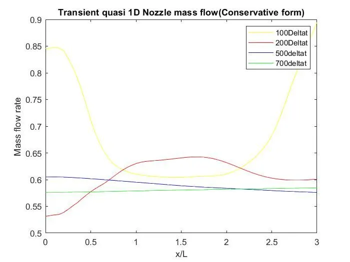
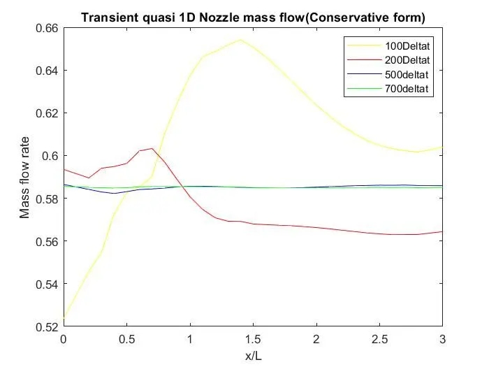
1) Mass flow rate vs (x/L) ratio for Transient quasi 1D Nozzle mass flow(Conservative form) for N = 61(FIRST PART) & N = 31(SECOND PART) nodes respectively
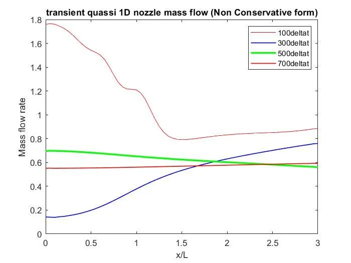
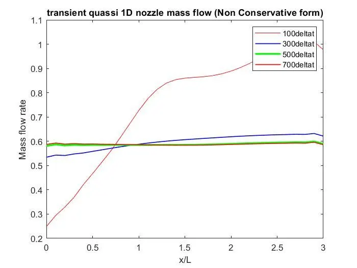
2) Mass flow rate vs (x/L) ratio for Transient quasi 1D Nozzle mass flow(Non Conservative form) for N = 61(FIRST PART) & N = 31(SECOND PART) nodes respectively
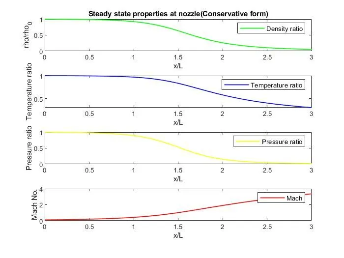
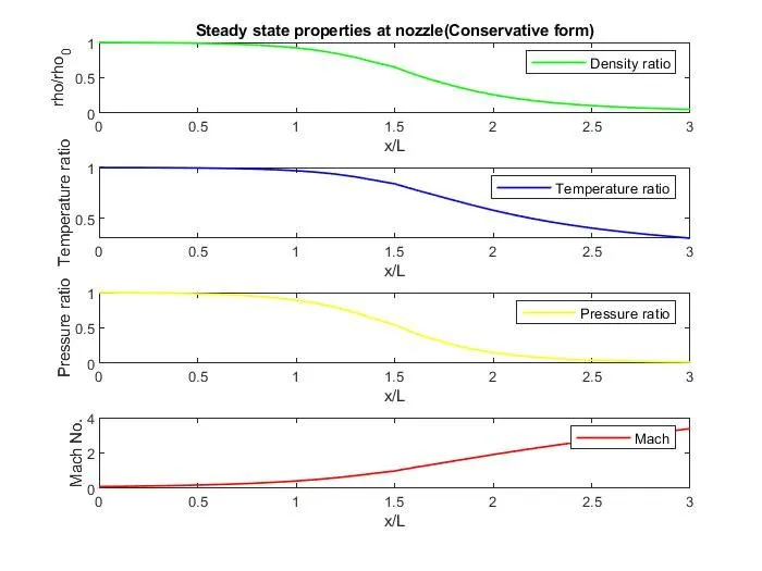
3) Steady state Properties vs (x/L) ratio for Transient quasi 1D Nozzle mass flow( Conservative form) for N = 61(FIRST PART) & N = 31(SECOND PART) nodes respectively
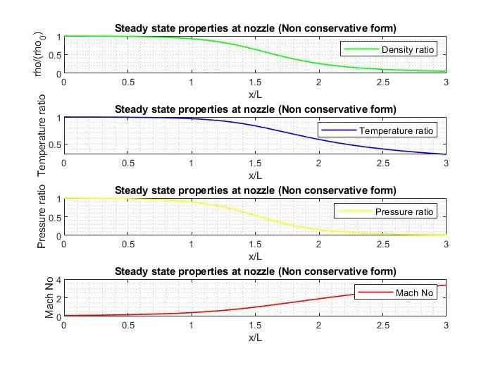
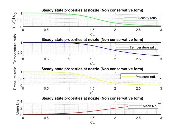
4) Steady state Properties vs (x/L) ratio for (Non Conservative form) for N = 61(FIRST PART) & N = 31(SECOND PART) nodes respectively
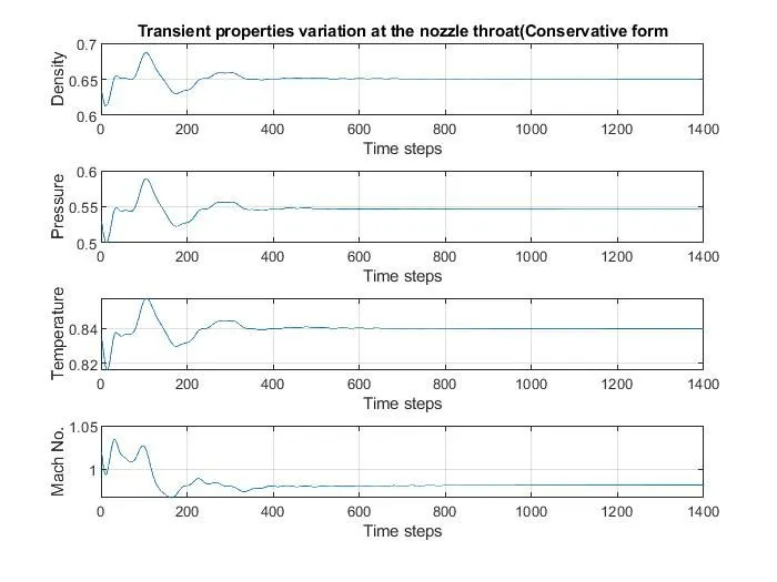
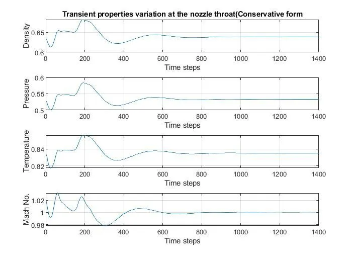
5) Transient state Properties vs (x/L) ratio for Transient quasi 1D Nozzle throat mass flow( Conservative form) for N = 61(FIRST PART) & N = 31(SECOND PART) nodes respectively
6) Transient state Properties vs (x/L) ratio for Transient quasi 1D Nozzle mass flow(Non Conservative form) for N = 61(FIRST PART) & N = 31(SECOND PART) nodes respectively
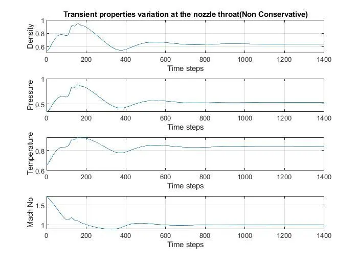
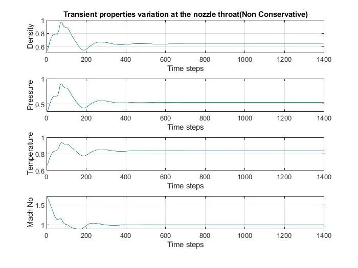
7) Transient state Properties vs (x/L) ratio for Transient quasi 1D Nozzle mass flow(Non Conservative form) for N = 61(FIRST PART) & N = 31(SECOND PART) nodes respectively
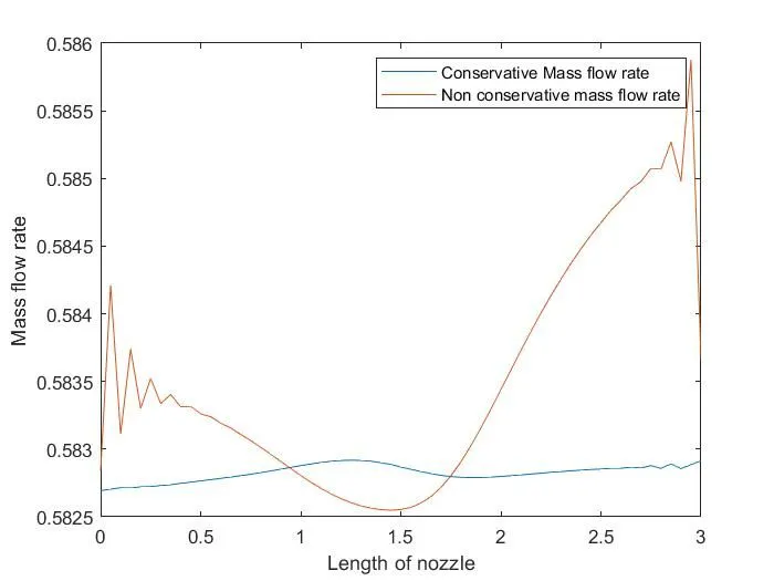
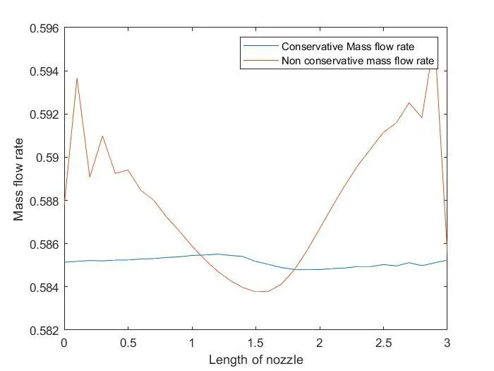
Observations:
- For a general understanding,the conservative form that the Eulers approach where the control volume is fixed and the properties of the fluid element passing through it are studied.Whereas the NonConservative form takes the lagrangian approach where certain fluid elements and their properties are studied along its path in the overall control domain.
- This gives an advantage to conservative form in the cases where there are sudden shocks in domain where the system of variables would undergo a very significant change in consecutive spatial domain.
- Although both the form make no differance when we approach them analytically.There is significant difference when we look at coding aspect of problem.
- In this problem solution converged much faster using conservative form,that conclusion can be drawn above plots.
- The first 4 plots(figure1&2) gives the insight of nondimensionalised mass flow rate vs time. Here different curves are shown each for different time during the time marching procedure. For transient state with 31 nodes & 61 nodes for both Conservative and non-Conservative form variation can be seen.
- The another set of 4 plots (figure3&4) is showing steady state properties in which no variation in steady state properties wrt node size can be seen for both Conservative and NonConservative nodes. Steady state propertis for Conservative and Nonconservative form results are similar in trend.
- Plot 7(figure13&14) irrespective of any no. of nodes Conservative form is giving stable solution as compared to Nonconservtie form.
- For this problem we can conclude that the conservative form has the also lead to more accurate and stable solution because the solution obtained is closer to analytical solution when compared with the nonconservative part.
Grid Indepedence Test:
In general when we perform any calculations using numerical methods we calculate as per governing eqautions across fixed node points.These nodes points essentially form grid/mesh.
As number of nodes increases the spatial difference between the point decreases and the solution obtained is more accurate.But this inturn increases overall computation time. Hence it is very necessary to arrive at value for number of nodes or basically, the mesh density for our physical domain under consideration so that we can estimate the solution to be within acceptable range of accuracy and save our computation time by not considering mesh with higher densities.
| Sr. No. | Type of Solution | Density | Temperature | Pressure | Mach Number |
| 1 | Analytical Solution | 0.634 | 0.833 | 0.528 | 1 |
| 2 | 61nodes- Conservative | 0.639 | 0.8355 | 0.5339 | 0.9979 |
| 3 | 61nodes-Nonconservative | 0.5917 | 0.8081 | 0.4782 | 1.0753 |
| 4 | 61nodes-Conservative | 0.6517 | 0.8407 | 0.5479 | .9792 |
| 5 | 0.5961 | 0.5961 | 0.8136 | 0.485 | 1.0867 |
Our code was begun with 61 node points and the above table gives us a picture of how the solutions obtained compare with the actual analytical solutions. The values are that of the primitive variables in the throat section of our domain.The analytical were obtained with reference from the textbook of CFD.
It becomes quite obvious that a higher number of nodes lead to a solution that is more accurate. But the solutions obtained from the mesh with 31 nodes were also reasonably accurate. Hence one can decide if one wants a high accuracy that would take more computational time or stop at a lower mesh density with slight compromise on the solution accuracy.