Week 5.1 - Mid term project - Solving the steady and unsteady 2D heat conduction problem
Week 5.1 - Mid-term project - Solving the steady and unsteady 2D heat conduction problem
Aim: Solve the 2D heat conduction (Steady +Transient) equation by using the point iterative techniques that were taught in the class. The Boundary conditions for the problem are as follows;
Top Boundary = 600 K
Bottom Boundary = 900 K
Left Boundary = 400 K
Right Boundary = 800 K
By implementing the following methods for solving implicit equations.
- Jacobi
- Gauss-seidel
- Successive over-relaxation
Steady state Heat Conduction:
It is type of heat conduction in which Temperature is not changing w.r.t time. General equation for steady state heat conduction can be given by,
`(∂^2 T)/(∂x^2 )+(∂^2 T)/(∂^2 y)= 0` (1)
Where T = Temperature (K), & x, y is space coordinate respectively
For steady state heat transfer is given by,
`∂T/∂t=0` (2)
If we discretize the above equation (1), final and simplified expression can be written as,
`T_P=1/k ((T_L+T_R)/(∆x^2 ))+1/k((T_T+T_B)/(∆y^2 ))` (3)
Now, applying the node in above equation (3), we will have
`T_(i,j)=1/k ((T_(i-1,j)+T_(i+1,j))/(∆x^2 ))+1/k((T_(i,j-1)+T_(i,j+1))/(∆y^2 ))` (4)
Now this above equation (4) can be solved by iterative methods which is mentioned in problem statement. Iterative method is mathematical procedure that uses the initial guess to initiate the problem and after certain iteration it will converge.
- Jacobi Method: It is iterative method in which all updated values are used for computations only after all the variables have updated.
Mathematically above eqn. (4) can be expressed by using Jacobi method,
`T_(i,j)=1/k ((〖T_old〗_(i-1,j)+〖T_old〗_(i+1,j))/(∆x^2 ))+1/k((〖T_old〗_(i,j-1)+〖T_old〗_(i,j+1))/(∆y^2 ))`
- Gauss-sidel Method: In this iteration method updated variables are used in computation as soon as they have updated.
Mathematically above eqn (4) can be expressed by using GS method,
`T_(i,j)=1/k ((〖T_old〗_(i-1,j)+T_(i+1,j))/(∆x^2 ))+1/k((〖T_old〗_(i,j-1)+T_(i,j+1))/(∆y^2 ))`
- Successive over-relaxation method: This iteration method is used for enhancing the performance of G-S method and Jacobi method.
If relaxation factor () < 1 underrelaxed
>1 overrelaxed
Now, applying SOR method for equation (4) we will have,
`T_(i,j)=(1-ω)*〖T_old〗_(i,j)+ω*[1/k ((〖T_old〗_(i-1,j)+T_(i+1,j))/(∆x^2 ))+1/k ((〖T_old〗_(i,j-1)+T_(i,j+1))/(∆y^2 ))]`
%Steady state 2D heat trasnfer Analysis %
clear all
close all
clc

%Defining inputs%
nx = 10; %No of grid points along x axis
ny = 10; %No of grid points along y axis

%Mesh information
x = linspace(0,1,nx);  % Discretization in x axis
y = linspace(0,1,ny);  % Discretization in y axis

%Mesh size

dx = x(2) -x(1);
dy = y(2)- y(1);

% To initilise the temperature
T = 300*ones(nx,ny);

%To apply boundary condition
T(1,:) = 600 ;%Top boundary
T(ny,:)= 900 ;%Bottom boundary
T(:,1) = 400; %Left boundary
T(:,nx)= 800; %Right boundary

%Generating temperature copy
Told = T;
Tinitial = T;
tol = 1e-4   %Given tolerance
error_jac = 9e9 % Initial guess

%Jacobi method

tic
jacobi_iter = 0;

%Convergence loop

while(error_jac > tol)

    %Space loop
    for i = 2:nx-1
        for j = 2:ny-1
            k = 2*(dx^2+dy^2)/(dx^2*dy^2);
            term1 = 1/k*(Told(i-1,j)+Told(i+1,j))/(dx^2);
            term2 = 1/k*(Told(i,j-1)+Told(i,j+1))/(dy^2);
            T(i,j) = (term1+term2);  %Jacobi iteration
        end
    end
    error_jac = max(max(abs(Told-T)));
    Told = T; %Updating the Told value
    jacobi_iter = jacobi_iter + 1;
end
toc
%Plotting
figure(1)
contourf(x,y,T)
clabel(contourf(x,y,T));
colorbar
colormap(jet)
xlabel('X axis')
ylabel('Y axis')
title_text = sprintf('Jacobi iteration number = %d',jacobi_iter');
title(title_text)
set(gca,'YDIR','reverse')


%Gauss sidel method%

tic
T = Tinitial ;
Told = Tinitial;
error_GS = 9e9;

%Convergence loop
GS_iter = 0;
while(error_GS > tol)

    %Space loop

     for i = 2:nx-1
        for j = 2:ny-1
            k = 2*(dx^2+dy^2)/(dx^2*dy^2);
            term1 = (T(i-1,j)+Told(i+1,j))/(dx^2);
            term2 = (T(i,j-1)+Told(i,j+1))/(dy^2);
            T(i,j) = 1/k*(term1+term2);  %GS iteration
        end
    end
    error_GS = max(max(abs(Told-T)));
    Told = T; %Updating the Told value
    GS_iter = GS_iter + 1;
end
toc
%Plotting
figure(2)
contourf(x,y,T)
clabel(contourf(x,y,T));
colorbar
colormap(jet)
xlabel('X axis')
ylabel('Y axis')
title_text = sprintf('GS iteration number = %d',GS_iter');
title(title_text)
set(gca,'YDIR','reverse')

%SOR Method %

tic
T = Tinitial ;
Told = Tinitial;
error_SOR = 9e9;
w = 1.2;
error = 1;


%Convergence loop
SOR_iter = 0;
while(error_SOR > tol)

    %Space loop

     for i = 2:nx-1
        for j = 2:ny-1
            k = 2*(dx^2+dy^2)/(dx^2*dy^2);
            term1 = (T(i-1,j)+Told(i+1,j))/(dx^2);
            term2 = (T(i,j-1)+Told(i,j+1))/(dy^2);
            T(i,j) = (1-w)*Told(i,j)+(w*(1/k)*(term1+term2));  %SOR iteration
        end
    end
    error_SOR = max(max(abs(Told-T)));
    Told = T; %Updating the Told value
    SOR_iter = SOR_iter + 1;
end
toc
%Plotting
figure(3)
contourf(x,y,T)
clabel(contourf(x,y,T));
colorbar
colormap(jet)
xlabel('X axis')
ylabel('Y axis')
title_text = sprintf('SOR iteration number = %d',SOR_iter');
title(title_text)
set(gca,'YDIR','reverse')
In the entire code following Procedure is been followed:
- Initial grid points along x and y axis were defined.
- Next mesh and mesh size were defined.
- Define initial and boundary condition.
- Creating copy of initial temperature.
- Error and tolerance values are defined for all the methods.
- Further iteration procedure for Jacobi, GS & SOR method is developed.
- Iteration method consists of two loops.
1)Space loop 2) Convergence loop
- Space loop consists of two loops to calculate Temperature T along both X and Y direction.
- This space loops are inside the convergence loop, which will execute its function till error is reach to value of tolerance given.
- Based on iteration method 2D Equation of T will very. After for loop error value is calculated & updated Told as T value.
- Next iteration no will also be updated.
Simulated Result: Contours of Jacobi, Gauss sidel and SOR method is shown below in sequence.
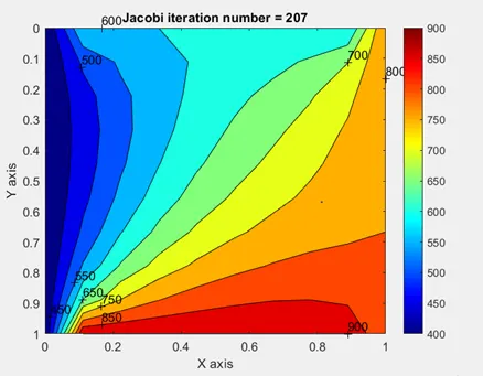
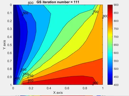
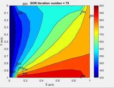
here we can say from above plots,
No of iterations will be Jacobi (207) > Gauss sidel(111) > SOR Method(75).
MATLAB Code for transient heat conduction (Explicit method):
%Unsteady state heat transfer using explicit method
clear all
close all
clc

%Defining the inputs %

nx = 10; %No of grid points along x axis
ny = 10; %No of grid points along y axis

%Mesh information
x = linspace(0,1,nx);  % Discretization in x axis
y = linspace(0,1,ny);  % Discretization in y axis

%Mesh size

dx = x(2) -x(1);
dy = y(2)- y(1);

% To initilise the temperature

T = 300*ones(nx,ny);

%To apply boundary condition
T(1,:) = 600 ;%Top boundary
T(ny,:)= 900 ;%Bottom boundary
T(:,1) = 400; %Left boundary
T(:,nx)= 800; %Right boundary

%Generating temperature copy
Told = T;
tol = 1e-4;
error = 10;
dt = 0.001;
alpha = 1.4;

%CFL no %
k1 = alpha*(dt/dx^2);  %CFL no for x direction
k2 = alpha*(dt/dy^2);  %CFL no for y direction

tic
iter = 1;
for nt= 1:1400;
    while(error>tol)

        %Space Loop%
        for i= 2:nx-1;
            for j = 2:ny-1;

                term1 = k1*(Told(i-1,j)-2*Told(i,j)+Told(i+1,j));
                term2 = k2*(Told(i,j-1)-2*Told(i,j)+Told(i,j+1));
                T(i,j)= T(i,j)+term1+term2; % Implicit method
            end
        end
        error = max(max(abs(Told-T)));
        Told = T; %Updating the old value
        iter = iter+ 1;
    end
end

%Plotting
figure(1)
contourf(x,y,T)
clabel(contourf(x,y,T));
colorbar
colormap(jet)
xlabel('X Axis')
ylabel('Y Axis')
title_text = sprintf('iteration number = %d',iter);
title(title_text)
set(gca,'YDIR','reverse')
toc
MATLAB Code explanation for transient heat conduction (Explicit method):
- Initial grid points along x and y axis were defined.
- Next mesh and mesh size were defined.
- Define initial and boundary condition.
- Creating copy of initial temperature.
- Error and tolerance values are defined for all the methods.
- For further iteration Explicit method is developed.
- Iteration method consists of three loops.
1)Time loop 2) Space loop 3) Convergence loop
- Time loop consists of one loop to calculate Temperature T along time step interval t.
- Space loop consists of two loops to calculate Temperature T along both X and Y direction.
- This space loops are inside the convergence loop, which will execute its function till error is reach to value of tolerance given.
- Next iteration no will also be updated.
Simulated Result:
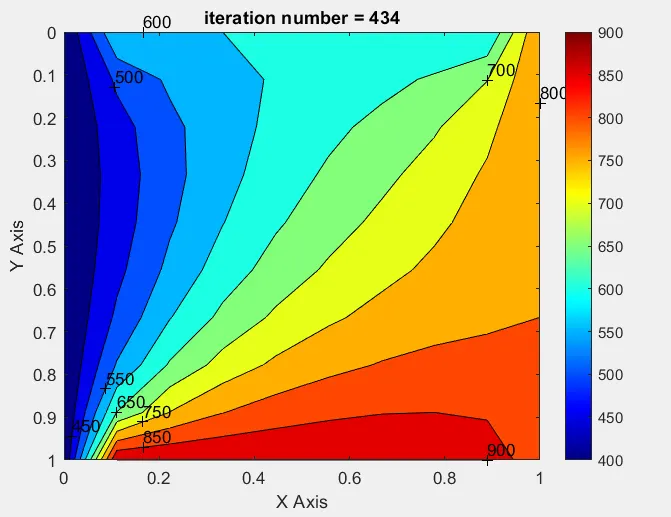
No. of iteration = 434
Error = 9.883610562155809e-05
CFL = 0.2268 (Formula is shown in MATLAB code)
Since CFL No. is less than 0.5 the solution is stable.
- Explicit method: This method uses future solution for corresponding future value.it is unconditionally stable.
- In this method iterative methods are used because all the values are unknown.
`T_P^(n+1)=〖1/(1+2k_1+2k_2 )*[T〗_P^n+k_1 (T_L+T_R )^(n+1)+k_2 (T_T+T_B )^(n+1) ]`
- Applying the node (i, j) in above equation,
`T_(i,j)^(n+1)=〖1/(1+2k_1+2k_2 )*[T〗_(i,j)^n+k_1 (T_(i-1,j)+T_(i+1,j) )^(n+1)+k_2 (T_(i,j+1)+T_(i,j-1) )^(n+1)]`
MATLAB Code for transient heat conduction (Implicit method):
%Unsteady state heat transfer using implicit method
clear all
close all
clc

%Defining the inputs %

nx = 10; %No of grid points along x axis
ny = 10; %No of grid points along y axis

%Mesh information
x = linspace(0,1,nx);  % Discretization in x axis
y = linspace(0,1,ny);  % Discretization in y axis

%Mesh size

dx = x(2) -x(1);
dy = y(2)- y(1);

% To initilise the temperature

T = 300*ones(nx,ny);

%To apply boundary condition
T(1,:) = 600 ;%Top boundary
T(ny,:)= 900 ;%Bottom boundary
T(:,1) = 400; %Left boundary
T(:,nx)= 800; %Right boundary

%Generating temperature copy
Told =T;
Tinitial = T;
Tprev = Told;

%Defining tolerance, alpha and time step
tol = 1e-4;
dt = 0.001;
alpha = 1.4;

%CFL Number %
%CFL no %
k1 = alpha*(dt/dx^2);  %CFL no for x direction
k2 = alpha*(dt/dy^2);  %CFL no for y direction
Iterative_solver = 3 ;
tic
%Implicit Jacobi method%
if Iterative_solver == 1
Imp_Jacobi_iter = 0;

%Time loop
for nt = 1:1400

    %Convergence loop
    error_jacobi = 9e9;
    while(error_jacobi> tol)

        %Space loop
        for i = 2:nx-1
            for j = 2:ny-1
                term1 = 1/(1+2*k1+2*k2);
                term2 = k1*term1;
                term3 = k2*term1;
                H = Told(i-1,j)+Told(i+1,j);
                V = Told(i,j-1)+Told(i,j+1);

                T(i,j) = (term1*Tprev(i,j))+(H*term2)+(V*term3);
            end
        end
        error_jacobi = max(max(abs(Told -T)));
        Told = T;  % Updating the Told value
        Imp_Jacobi_iter = Imp_Jacobi_iter +1;
    end
    Tprev = T;
end
toc
%Plotting%
figure(1)
contourf(x,y,T)
clabel(contourf(x,y,T));
colorbar
colormap(jet)
xlabel('X Axis')
ylabel('Y Axis')
title_text = sprintf('Implicit jacobi iteration number = %d',Imp_Jacobi_iter);
title(title_text)
set(gca,'YDIR','reverse')
end

%Implicit Gauss sidel method%
if Iterative_solver == 2
Imp_GS_iter = 0;

%Time loop
for nt = 1:1400

    %Convergence loop
    error_GS = 9e9;
    while(error_GS> tol)

        %Space loop
        for i = 2:nx-1
            for j = 2:ny-1
                term1 = 1/(1+2*k1+2*k2);
                term2 = k1*term1;
                term3 = k2*term1;
                H = T(i-1,j)+Told(i+1,j);
                V = T(i,j-1)+Told(i,j+1);

                T(i,j) = (term1*Tprev(i,j))+(H*term2)+(V*term3);
            end
        end
        error_GS = max(max(abs(Told -T)));
        Told = T;  % Updating the Told value
        Imp_GS_iter = Imp_GS_iter +1;
    end
    Tprev = T;
end
toc
%Plotting%
figure(2)
contourf(x,y,T)
clabel(contourf(x,y,T));
colorbar
colormap(jet)
xlabel('X Axis')
ylabel('Y Axis')
title_text = sprintf('Implicit GS iteration number = %d',Imp_GS_iter);
title(title_text)
set(gca,'YDIR','reverse')
end

    %Implicit SOR method%
    if Iterative_solver == 3
    w = 1.1;
Imp_SOR_iter = 0;

%Time loop
for nt = 1:1400

    %Convergence loop
    error_SOR = 9e9;
    while(error_SOR> tol)

        %Space loop
        for i = 2:nx-1
            for j = 2:ny-1
                term1 = 1/(1+2*k1+2*k2);
                term2 = k1*term1;
                term3 = k2*term1;
                H = T(i-1,j)+Told(i+1,j);
                V = T(i,j-1)+Told(i,j+1);

                T(i,j) = (1-w)*Told(i,j)+w*((term1*Tprev(i,j))+(H*term2)+(V*term3));
            end
        end
        error_SOR = max(max(abs(Told -T)));
        Told = T;  % Updating the Told value
        Imp_SOR_iter = Imp_SOR_iter +1;
    end
    Tprev = T;
end
toc
%Plotting%
figure(3)
contourf(x,y,T)
clabel(contourf(x,y,T));
colorbar
colormap(jet)
xlabel('X Axis')
ylabel('Y Axis')
title_text = sprintf('Implicit SOR iteration number = %d',Imp_SOR_iter);
title(title_text)
set(gca,'YDIR','reverse')
    end
MATLAB Code explanation for transient heat conduction (Implicit method):
- Initial grid points along x and y axis were defined.
- Next mesh and mesh size were defined.
- Define initial and boundary condition.
- Creating copy of initial and previous temperature.
- Error and tolerance values are defined for all the methods.
- For further iteration Jacobi, GS & SOR method is employed.
- Iteration method consists of three loops.
1)Time loop 2) Space loop 3) Convergence loop
- Time loop consists of one loop to calculate Temperature T along time step interval t.
- Space loop consists of two loops to calculate Temperature T along both X and Y direction.
- This space loops are inside the convergence loop, which will execute its function till error is reach to value of tolerance given.
- Next iteration no will also be updated.
- Here in this code iteration solver concept is used. Here 3 Iteration solver is present which is Jacobi, GS & SOR respectively. Now if iteration solver = 1 is selected then Jacobi method is executed. Simillarly for GS & SOR 2, 3 value is given into iteration solver to execute into MATLAB.
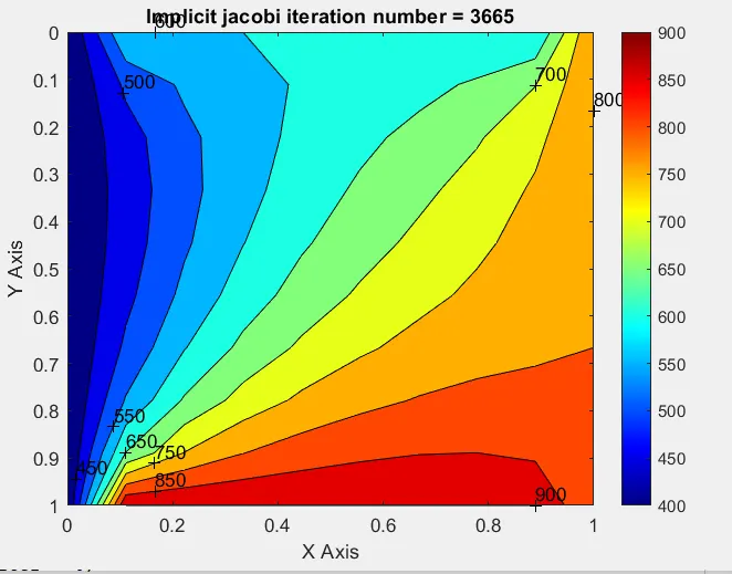
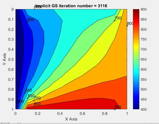
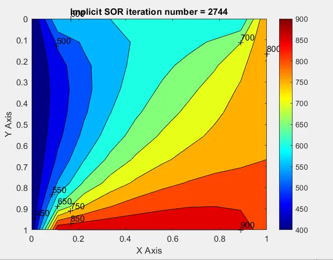
Simulated Result:
Iterations:
In terms of iteration, No of iteration taken by each iterative method is,
Jacobi(3665) > GS(3116) > SOR(2744) .
For both steady state and unsteady state SOR method is converged faster than Jacobi and GS Method. Jacobi method takes more time as compare to all other method.