A mathematical approach to Explicit and Implicit Analysis in FEA

AIM: To perform mathematical implicit and explicit analysis on the given cubic force-displacement equation for a tensile operation and discuss the difference in results obtained.

Problem description: The present problem is related to a tensile expansion of a simple bar as shown below:

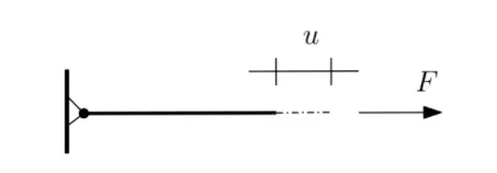
The external force applied is denoted as F, displacement is denoted as u and internal force experienced is given as f.

The force-displacement equation is given as :

F = K u

When force is varying, we get

`Delta F = K Delta u`

The given equation for displacement is:

`f(u)= u^3 + 9 u^2 + 4u`

Using the force-displacement relation, we can also obtain the stiffness relation:

`K = frac{df}{du} = 3 u^2 + 18 u +4`

Explicit analysis: In an explicit analysis, we take the given displacement equation for force and use incremental load steps onto it. For example, use increments of 1 unit of force `Delta F = 1`. This causes incremental changes to displacement and using that the stiffness and internal force can be calculated. For an ideal scenario with static equilibrium, the values for external force and internal force should be equal.

Explicit analysis is widely used in several FEA software for analysis of various applications. Typical applications include dynamic and quasi-static analysis. Examples for explicit analysis software include RADIOSS and LS Dyna. Generally, these applications have large deformations and time step is very small. Computational cost per time step is small.

Implicit analysis: In implicit analysis, the initial steps are the same as in explicit analysis. Incremental changes are given to the load and this results in incremental changes to displacement which can be used to calculate stiffness and internal forces. However, whenever internal force and external force are found to have large discrepancies > `10^-2`, Newton-Raphson iteration method is used to minimize the residual.

Implicit analysis is also used in FEA software for applications such as static and quasi-static analysis. Examples for implicit analysis software include ABAQUS and Nastran. Generally these applications have small deformation and time step used is large because computational cost per time step is large.

SOLUTION:

1. Explicit analysis: In explicit analysis, an incremental load of `Delta F = 1` is applied and the results obtained to displacement and internal force are noted down in three steps as follows:

Step 1: `Delta F = 1 , u0 = 0, K( u0 ) = 4`

`Delta u1 = (Delta F )/ (K(u0)) =1/4 = 0.25`

`u1 = u0 + Delta u1 = 0 + 0.25 = 0.25`

`u1 = 0.25`

`f = u^3 + 9 u^2 + 4 u = 1.578`

F = 1

R = f - F = 0.578

Step 2: `Delta F =1 , u1 = 0.25 , K(u1) = 8.6875`

`Delta u2 = (Delta F)/(K(u1)) = 1/8.6875 = 0.1151`

`u2 = u1 + Delta u2 = 0.25 + 0.1151 = 0.3651`

f = 2.708 , F = 2, R = f-F = 0.708

Step 3: `Delta F = 1, u2 = 0.3651, K(u2) = 10.9716`

`Delta u3 = (Delta F)/(K(u2)) = 1/10.9716 = 0.0911`

`u3 = u2 + Delta u3 = 0.3651 + 0.0911 = 0.4562`

f = 3.7928 , F = 3 , R = 0.7928

The results obtained by the explicit analysis can be summarized in the following table:

Steps	ΔF	F	Δu	u	f	R
1	1	1	0.25	0.25	1.578	0.578
2	1	2	0.1151	0.3651	2.708	0.708
3	1	3	0.0911	0.4562	3.7928	0.7928

As can be seen, the difference between internal force and the external force is high resulting in high residual values. This is not good because the system will not be stable statically.

2. Implicit analysis: Implicit analysis is similar to explicit at the beginning. But if the residual value is greater than `10^-2`, then Newton-Raphson iteration has to be used to bring down the residual value as shown in the steps below:

Step 1: `Delta F = 1, u0 = 0, K(u0) = 4`

`Delta u1 = (Delta F)/(K(u0)) = 1/4 = 0.25`

u1 = 0.25

f = 1.578, F = 1

R = f-F = 0.578

R> `10^-2`, therefore Newton-Raphson iteration has to be applied.

Iteration 1: `delta u ^(j+1) = -R^j/(K(u^j))`

`delta u^((1)) = -0.578/8.6875 = -0.0665`

`u1^((1)) = u1^((0)) + delta u1^((1)) = 0.25 - 0.0665 = 0.1834`

f = 1.0424

R=0.0424

R> `10^-2`, therefore Newton-Raphson iteration has to be applied again.

Iteration 2:

`delta u^((2)) = -0.0424/7.4021 = -0.005728`

`u1^((2)) = u1^((1)) + delta u2^((2)) = 0.1834-0.005728 = 0.1776`

f = 0.9998

R = 0.0002

Step 2: `Delta F =1 , u1 = 0.1776, K(u1) = 7.2914`

`Delta u2 = (Delta F)/(K(u1)) = 1/7.2914 = 0.1371`

`u2 = u1 + Delta u2 = 0.1776+0.1371 = 0.3147`

f = 2.1812

R = 0.1812

R> `10^-2`, therefore Newton-Raphson iteration has to be applied.

Interation 1:

`delta u2^((1)) = -0.1812/9.9617 = -0.0181`

`u2^((1)) = 0.3147 - 0.0181 = 0.2966`

f = 2.004236

R = 0.004236

Step 3: `Delta F = 1, u2 = 0.2966, K(u2) = 9.6027`

`Delta u3 = (Delta F)/(K(u2)) = 1/9.6027 = 0.1041`

`u3 = 0.2966 + 0.1041 = 0.4007`

f = 3.1121

R = 0.1121

R> `10^-2`, therefore Newton-Raphson iteration has to be applied.

Iteration 1:

`delta u3^((1)) = -0.1121/11.6942 = -0.0095`

`u3^((1)) = 0.4007 - 0.0095 = 0.3911`

f = 3.0009

R = 0.0009

The results obtained by implicit analysis are given below:

Steps	ΔF	F	Δu	u	f	R
1	1	1	0.1776	0.1776	0.9998	0.0002
2	1	2	0.122	0.2996	2.0042	0.0004
3	1	3	0.0915	0.3911	3.0009	0.0009

The residual values are very low meaning that the internal force and external force are almost equal.

As can be seen from the calculations, the implicit analysis will require more computation when compared to explicit analysis. At the cost of computational resources, the implicit analysis will have a more accurate result. Therefore, depending on application engineers can opt between using Implicit or Explicit analysis.

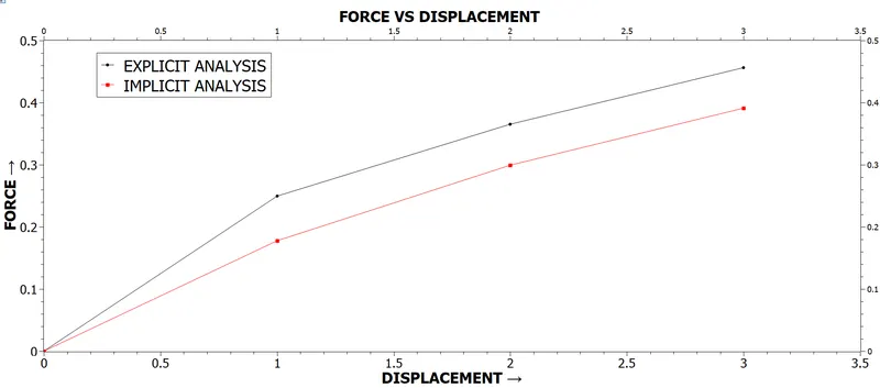
From the force vs displacement graph shown above, it can be seen that for the same force applied, the explicit analysis is giving higher values for displacement when compared to implicit analysis. From the tables, it can also be seen that explicit analysis gives higher residual values when compared to implicit.

Therefore, from an accuracy point-of-view, implicit analysis is better. However, in cases of large deformations with a very large number of nodes, implicit analysis can take a very long time and a lot of computational resources. Therefore, there is no objective superior mode of analysis. The engineer has to select the type of analysis based on the application, time allotted and computational resources available.

CONCLUSION: The explicit and implicit analyses for a simple rod undergoing tensile load was performed. The results were compared and discussion was made with regards to their application in the field of finite element analysis.