Week 10 - MRF project
Aim: To understand the MRF approach for predicting accurately the flow features in the given CAD object.
Introduction:
The Moving Reference Frame (MRF) approach is a steady-state method employed in industrial Computational Fluid Dynamics (CFD) to model problems with rotating parts. It is considered to be less computationally expensive and yet accurate enough for most industrial problems. For example, the rotors on a quadcopter can be modeled with MRFs.
For solving turbomachinery problems using CFD there exists specific and special models to be applied, and one of the models being popular in use is the Moving Reference Frame model. In MRF model a moving reference frame permits an unsteady problem (with respect to the absolute reference frame) to become steady in respect to the moving reference frame. In other words the complete rotor domain is assumed to be rotating at the same angular velocity of the rotor. Since basically all turbomachinery flows are unsteady in nature, the moving reference frame model approach makes simpler to solve these problems in CFD. It makes it easier to specify appropriate boundary conditions requiring less time and computational efforts and therefore is the preferred choice in industrial practices over rest of the models.
When a moving reference frame is activated, the equations of motion are modified to incorporate the additional acceleration terms i.e., Coriolis and centripetal acceleration terms which occur due to the transformation from the stationary to the moving reference frame. By solving these equations in a steady-state manner, the flow around the moving parts can be modeled.
Procedure:
Step 1: Simplifying the geometry.
The given .tzr file is unpacked in the icepak and several assemblies are created for simplifiction.
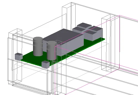
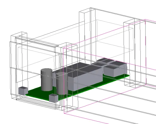
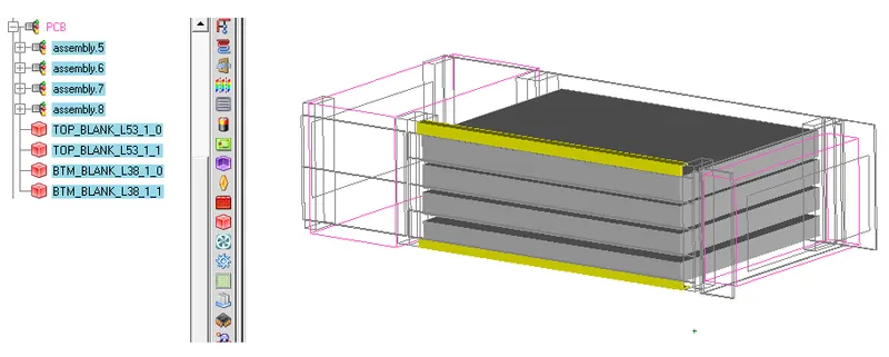
Two separate assemblies containing PCB, capacitors, power modules, panel holders are created. Along with these two assemblies, top blanks and bottom blanks, another assembly is created in the power module assembly.
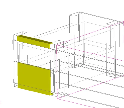
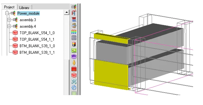
Beside this Power module assembly, there are 4 PCB's which is placed one above the other. Separate assemblies for each row are created. Combining all assemblies in another assembly along with two top and bottom blanks. All four assemblies along with two top and bottom blanks, another assembly is created and named PCB. as shown below.
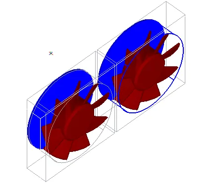
The fans available in the Icepak are not used in this simulation. Instead, fans are modeled separately taking care of all the important parameters such as blade angles at the inlet and exit and the rotor diameter. Along with Fans, the cutouts are modeled as fluid are used in this model.
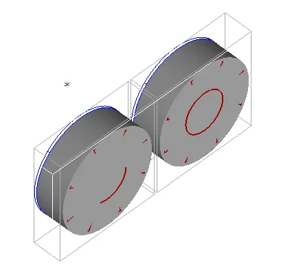
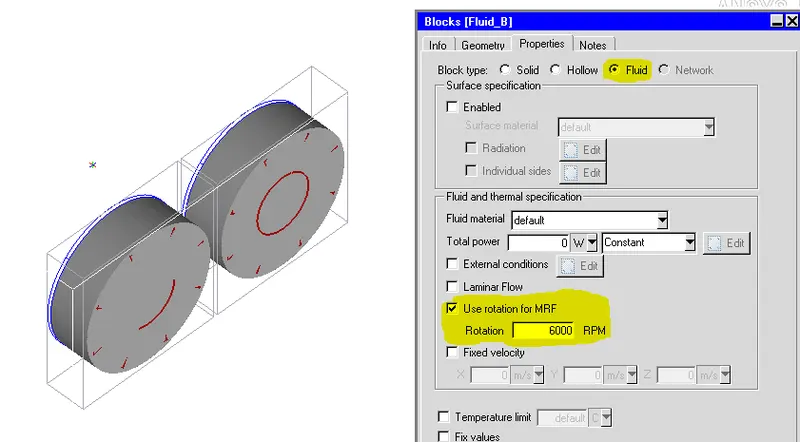
Fluid region are modeled and this is the important step in the icepak where the details about the MRF are given. For this problem, the rotation of 6000 rpm is given as the input as shown below.
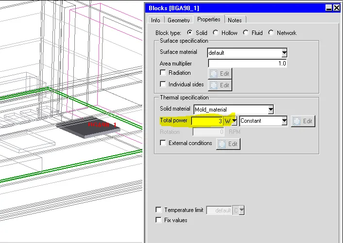
One of the BGA packs used in the PCB assembly has power input of 3W as shown below.
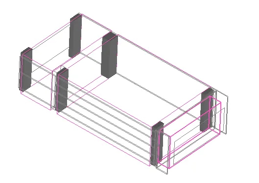
Few beams are provided in the cabinet used as a supporting structure.
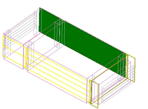
A big PCB is provided on the back side of the assemblies as shown below.
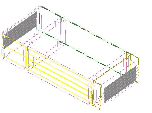
Sevaral openings were given in the model. But instead of considering the openings, two grilles are also provided on the front and rear end of the cabinet
Step 2: Meshing
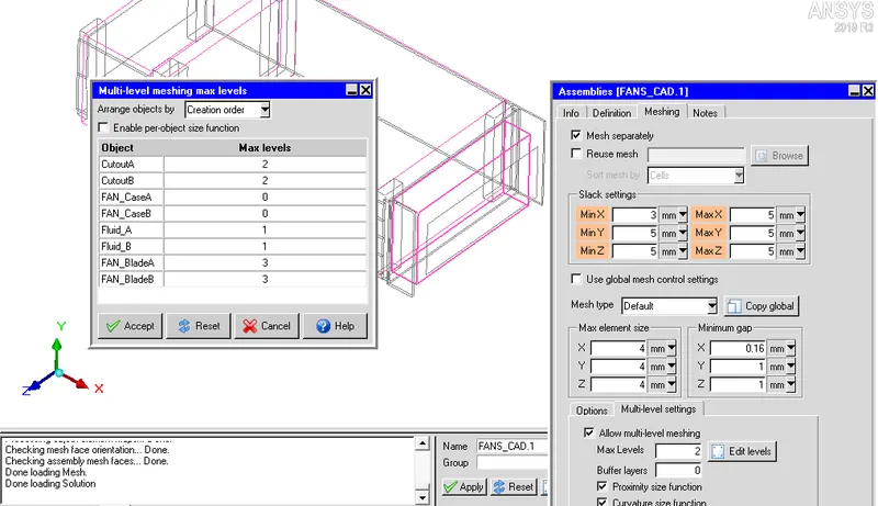
Meshing is an important part in any analysis. A non-conformal meshing is created by giving slack values for the assemblies and multilevel meshing is created for the fan object with 2 levels of meshing.
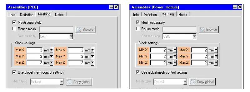
Also, for PCB and Power module, slack settings are given as 2 mm in all the directions.
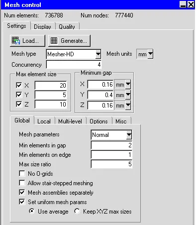
Mesh type : Mesher-HD is used with concurrency of 4. This concurrency of 4 with parallel computing helps in reducing the computation time when a model has more assemblies. Approximately 0.7 million elements were generated by specifying the maximum sizes of elements in X, Y and Z directions respectively as 20,5 and 10.
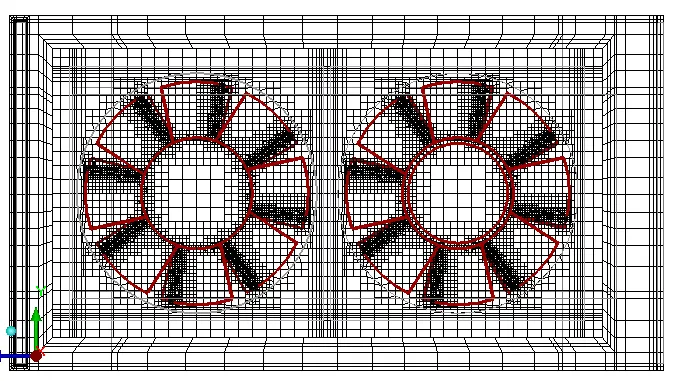
Below figure shows the surface mesh in both the fans.
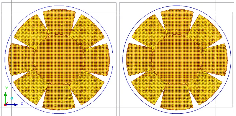
The cut plane mesh clearly shows the multilevel meshing achieved in the fans. here, fine mesh is created near the surface and is gradually increased away from the surface. this will reduce the mesh count without leaving the details near the surface.
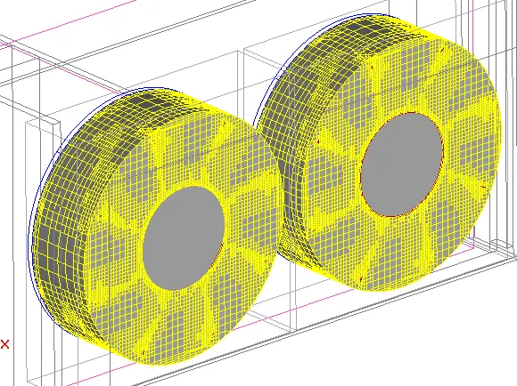
Also, surface mesh in the Fluid A and Fluid B clearly depicts the multilevel meshing
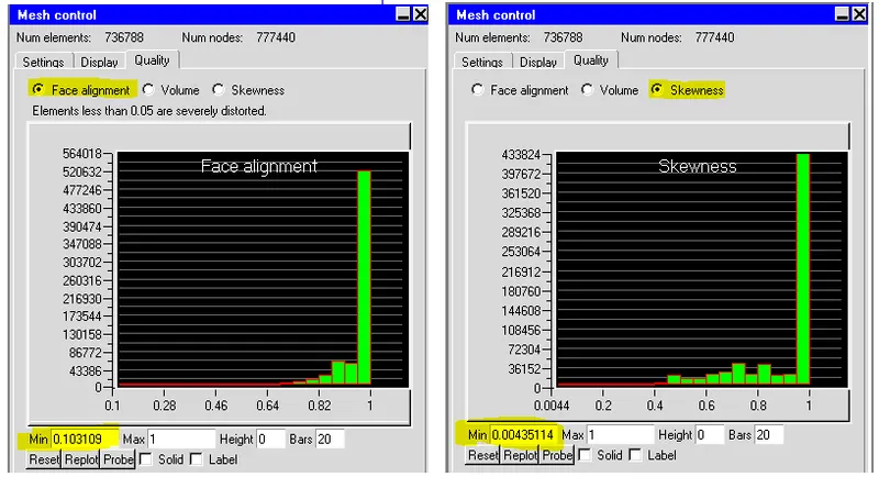
The quality of the mesh is found to be nearly good, hence proceeding with the simulation.
Step 3: Problem and solver settings
The problem is solved for forced convection with Realizable two equation turbulent model under state conditions without radiation. The ambient conditions are considered to be 20oC.
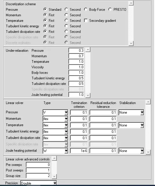
Under solver settings, double precision solver is used along with that, the first order discretization scheme is used for all the variables viz. pressure, momentum, temperature, turbulent kinetic energy and turbulent dissipation rate.
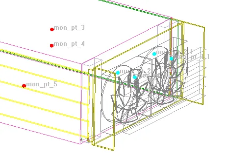
Monitor points are created on few of the edges and surfaces for monitoring velocity and temperture. Blue dots indicate velocity monitor points and Red dots indicate temperature monitor points.
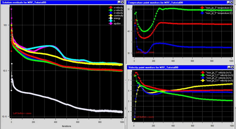
The convergence plot, temperature and velocity plots are shown below. It looks that solution is almost converged. the temperature and flow has attained steady state.
Step 5: Results and Discussion
Velocity plot:
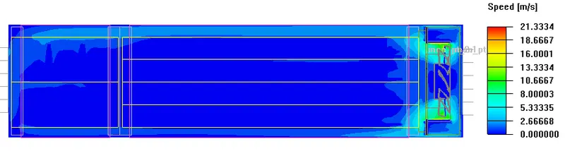
It is seen from the velocity plot that the highest velocity attained is 21 m/s approx. The fluid moves on top and bottom of the cabinet with higher velocities compared to the middle of the cabinet. This is clearly seen because of the MRF model. If normal fan is used with out MRF, then the flow conditions may not be accurate as the flow happens in the normal direction of the object.
Temperature plot:
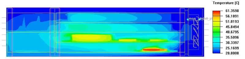
The location of the plane is in the middle of the cabinet in z-direction. It is seen from the temperature plot that the maximum temperature attained is 61.35oC which is in the operating range.
Particle track from the fans
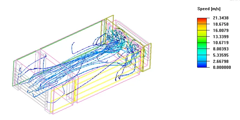
The particle track from the fans is shown above.
The above link shows the particle track animation.
Conclusion:
The MRF approach gives or predicts better information about the particle movements, temperature and velocity distribution in the vicinity of the fan when compared with the normal fan available in ICEPAK library.