Week 1- Mixing Tee

AIM: - To set up steady-state simulations to compare the mixing attentiveness when hot inlet temperature is 36 C and the cold inlet is at 19 C for a mixing tee problem using ANSYS FLUENT.

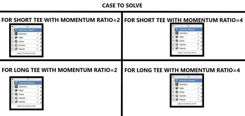
The cases to be simulated are as follows,

• Use k-epsilon & k-omega SST turbulence model for the first case and select the suitable model for further cases.
• Different mesh sizes 10mm,5mm, and 3mm for the second case and select the suitable model for further cases.
• Case 1- Short mixing tee with a hot inlet velocity of 3m/s and momentum ratio of 2 & 4
• Case 2:-Long mixing tee with a hot inlet velocity of 3m/s and momentum ratio of 2 & 4

OBJECTIVE

• To compare the cell count, average outlet temperature, and number of iterations tor convergence tor the given two case studies
• To perform mesh independent study for any one of the case studies,
• To use contour & line plots to study the output values of velocity and temperature along and across the length of the pipe

THEORETICAL EXPLANATION: -

The CFD Simulations of such setup are very important in practical applications like nuclear reactors, As When there is a large temperature difference between two fluid streams large temperature fluctuations can occur, which will lead to thermal fatigue of the piping system. Especially in the case of these tee connections temperature mixing effects cannot be accurately monitored by the mechanical

The turbulence model is the mathematical model to predict the effects of turbulence One of the most commonly used models RANS stands for Reynolds-Averaged Navier Stokes model. The k-E and kw models come under the RANS models of two-equation types. The two-equation type RANS models contain two transport equations for two turbulence properties which are turbulence kinetic energy and the dissipation rate of turbulence kinetic energy or the specific dissipation rate u The k-E the model has a modified version called realizable k-end similarly the k-o model has a more advanced version called k-omega Shear Stress Transport (SST) model

GOVERNING EQUATIONS

The temperature of the mixture is

Where T is the temperature of the fluid and m is the mass flow rate

`m=rho.A.v`

Where

`rho` is the density of the fluid

A is the cross-sectional area and

v is the velocity of the fluid

m hot=(1.225*.000901*3)= 0.003311

momentum ratio(M) = (Velocity at the cold inlet)/(Velocity at the hot inlet)

For M=2

`m cold=(1.225*.000225*6)= 0.001653.`

`Tmix=((0.003311*36)+(0.001653*19))/(0.003311+0.001653)`

Tmix= 30.311^0 C

For M=4

m cold=(1.225*.000225*12)= 0.003307

`Tmix=((0.003311*36)+(0.003307*19))/(0.003311+0.0.003307)`

`Tmix= 27.475^0 C`

PROCEDURE: -

*The model is been downloaded and added to the fluent workbench and the geometry is been checked in the space claim.

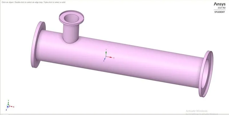
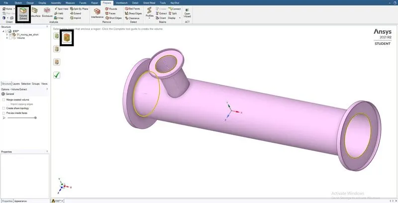
*The required area is volume extracted by selecting the edges of the inlets and outlet.

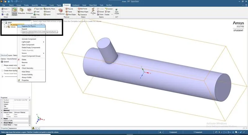
* The unwanted surface is suppressed to physics.

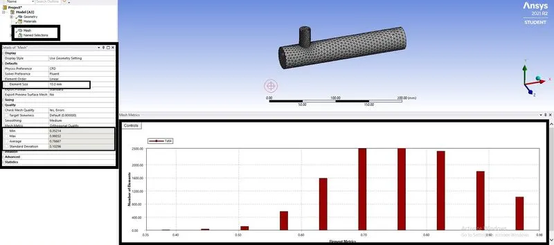
*The mesh is created for an element size of 10mm and the quality of the elements we more than 40%.

*The Setup workbench is started and given recommended parameters.

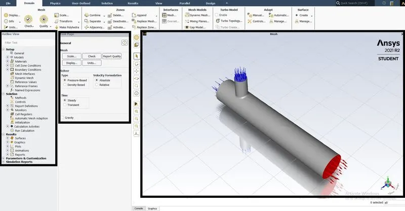
*The energy was turned on and turbulent model with k epsilon

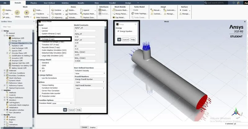
*The material is been added, the air is been initiated with specific values at both the inlets.

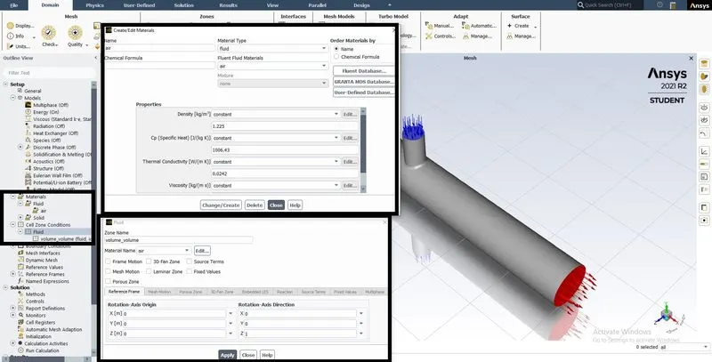
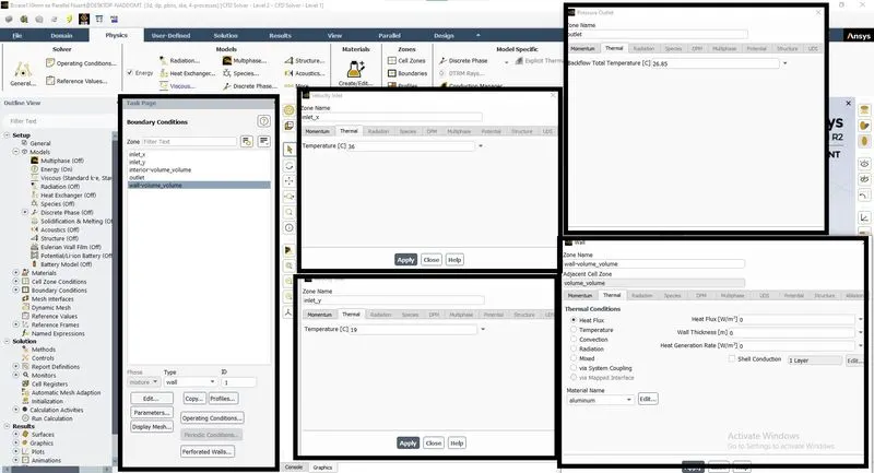
*Boundary Conditions are applied on the inlet in x and y with velocity values, outlet with pressure at zero, and the wall with No-slip conditions.

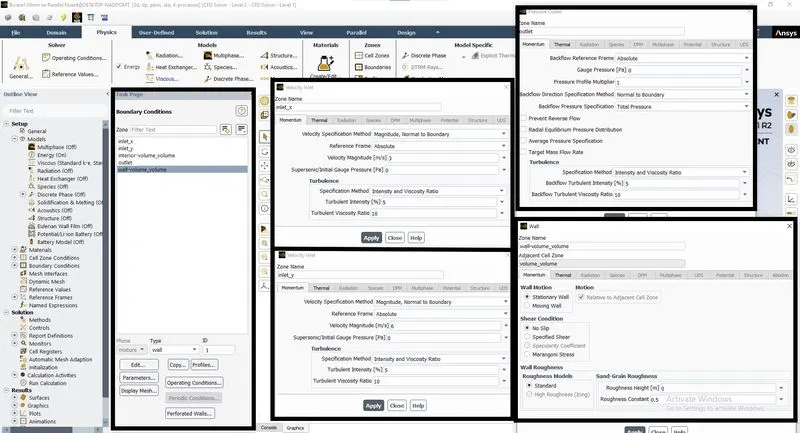
*Boundary Conditions are applied on the inlet in x and y with temperature values, outlet with the temperature at ambient condition.

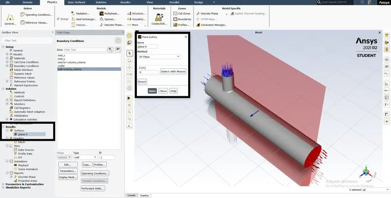
*The plane is created in XY direction to demonstrate the contours of pressure and temperature

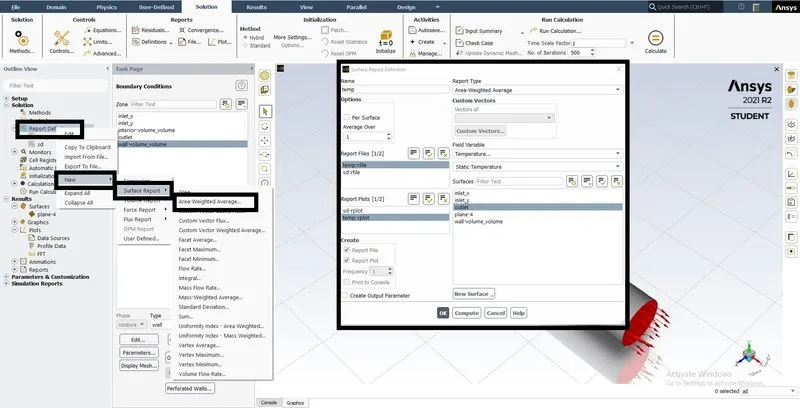
*Report definition is done by creating a surface report of Area weighted average for temperature and standard deviation at the outlet.

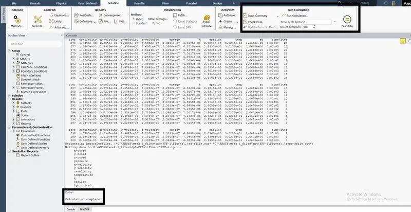
*The case is run to check for no of iterations and errors in the model setup.

*The residuals, surface report of Area weighted average for temperature, and standard deviation at the outlet are plotted to show the model has reached convergence.

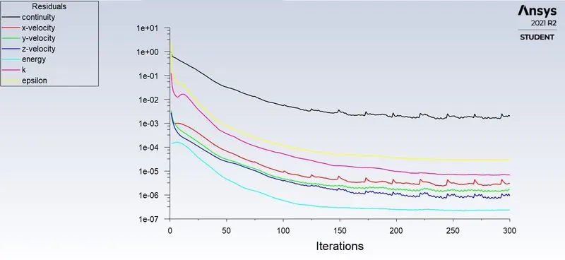
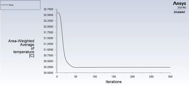
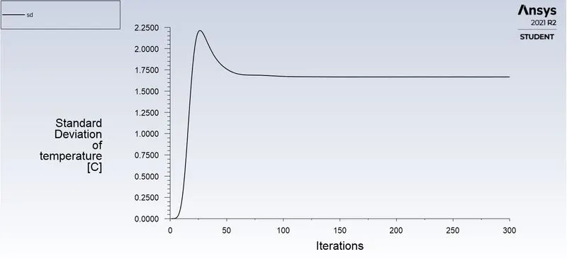
*The case is been initiated for mesh size 10mm for turbulent models K epsilon and K omega conditions.

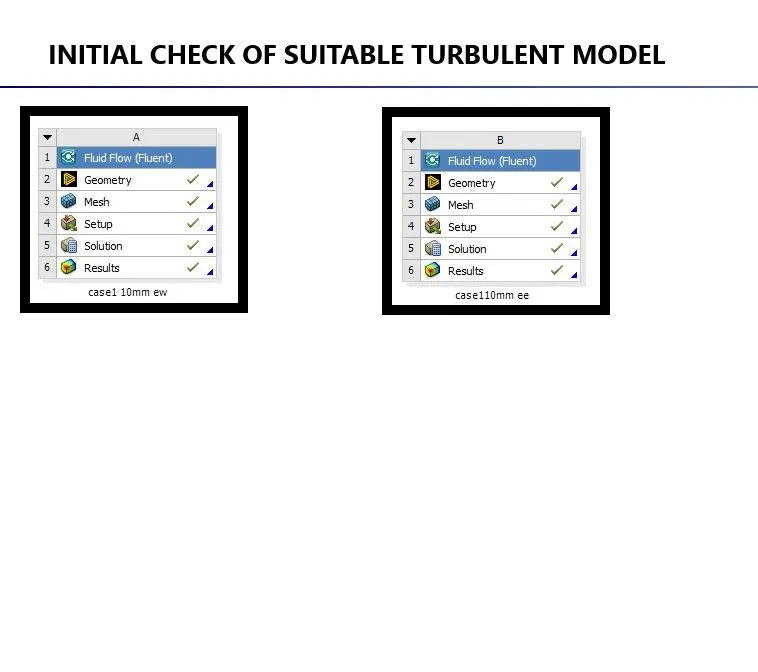
*The energy was turned on and turbulent model with k epsilon

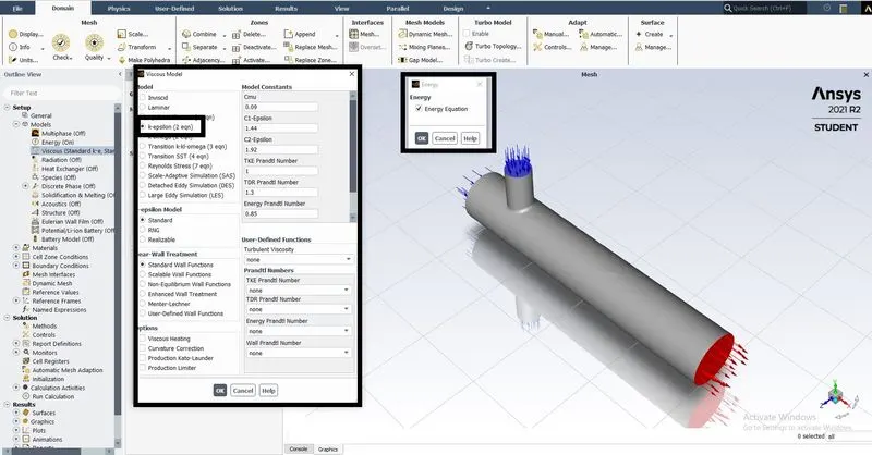
*The residuals, surface report of Area weighted average for temperature, and standard deviation at the outlet are plotted to show the model has reached convergence.

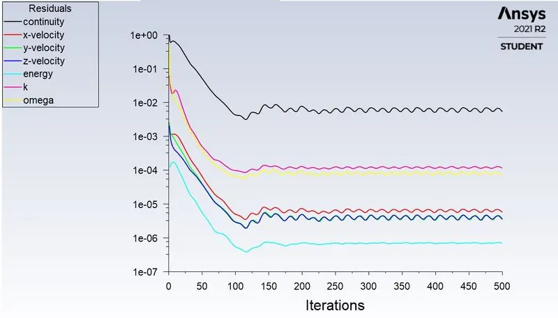
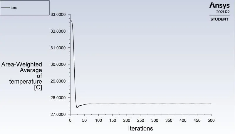
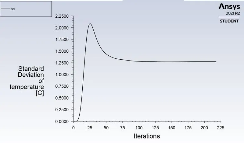
*The Turbulence model type check is done by comparing the following

TURBULENT MODEL	K EPSILON	K OMEGA
TEMPERATURE IN CELSIUS	30.27	30.23
STANDARD DEVIATION	1.443	1.667
NUMBER OF ITERATION TO REACH CONVERGENCE	297	800

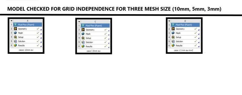
*The case is been initiated for different mesh sizes of 10mm, 5mm, and 3mm for turbulent models K epsilon model.

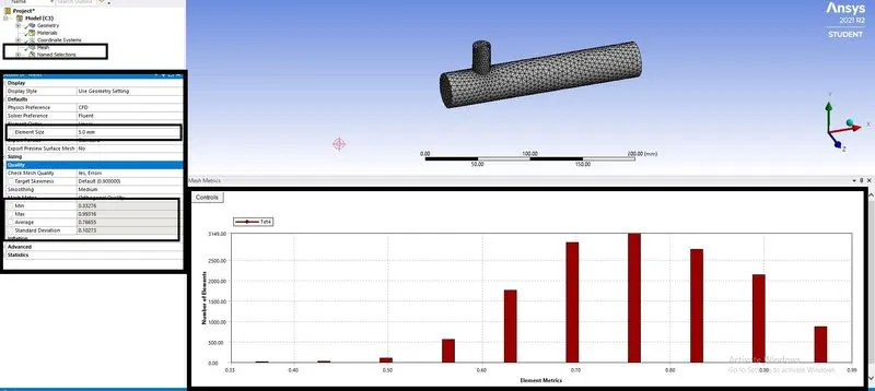
*The mesh is created for an element size of 5mm and the quality of the elements we more than 40%.

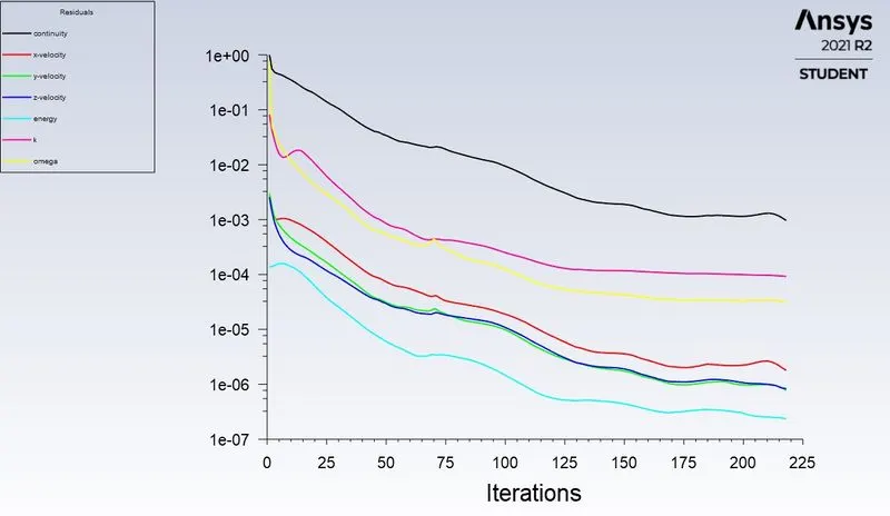
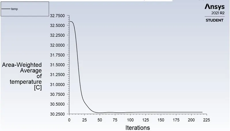
*The residuals, surface report of Area weighted average for temperature, and standard deviation at the outlet are plotted to show the model has reached convergence.

*The mesh is created for an element size of 3mm and the quality of the elements we more than 40%.

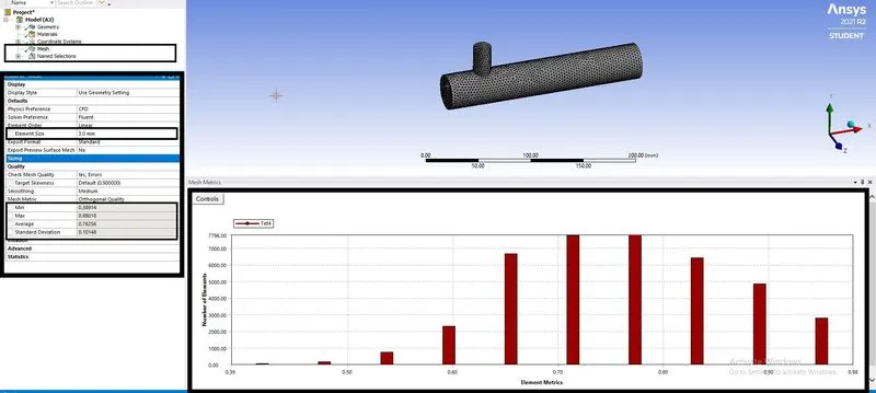
*The residuals, surface report of Area weighted average for temperature, and standard deviation at the outlet are plotted to show the model has reached convergence.

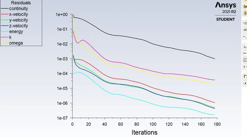
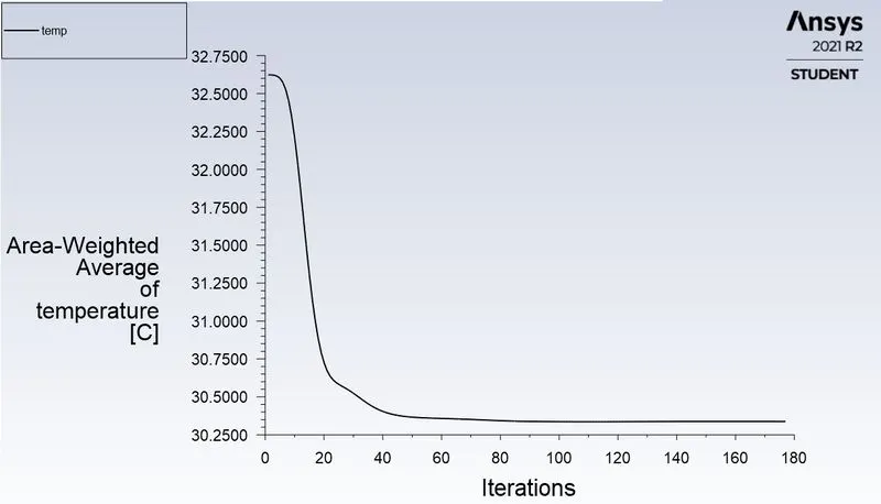
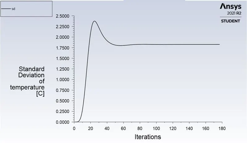
*The grid independence is done by comparing the following

GRID INDEPENDENCE	MESH SIZE 10mm	MESH SIZE 5mm	MESH SIZE 3mm
TEMPERATURE IN CELSIUS	30.27	30.294	30.3373
STANDARD DEVIATION	1.443	1.27355	1.8261
NUMBER OF ITERATION TO REACH CONVERGENCE	297	184	177

*The case is been initiated for different Mixing tee, mesh size 3mm for turbulent models K epsilon model.

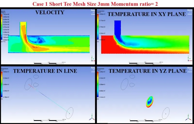
*Boundary Conditions are applied on the short tee inlet in x and y with velocity values of 3 and 6 for momentum ratio =2, outlet with pressure at zero, and the wall with No-slip conditions.

*The results have been plotted for Velocity and the temperature in XY plane, YZ plane, and line in XY plane.

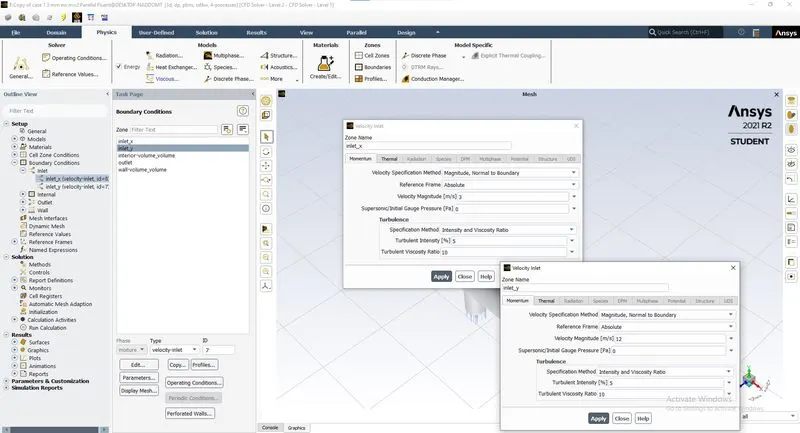
*Boundary Conditions are applied on the short tee inlet in x and y with velocity values of 3 and 12 for momentum ratio =4, outlet with pressure at zero, and the wall with No-slip conditions.

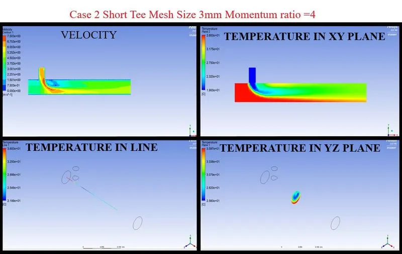
*The results have been plotted for Velocity and the temperature in XY plane, YZ plane, and line in XY plane.

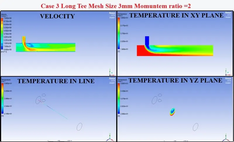
*Boundary Conditions are applied on the long tee inlet in x and y with velocity values of 3 and 6 for momentum ratio =2, outlet with pressure at zero, and the wall with No-slip condition.

*The results have been plotted for Velocity and the temperature in XY plane, YZ plane, and line in XY plane.

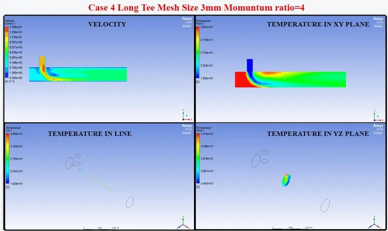
*Boundary Conditions are applied on the long tee inlet in x and y with velocity values of 3 and 12 for momentum ratio =4, outlet with pressure at zero, and the wall with No-slip conditions.

*The results have been plotted for Velocity and the temperature in XY plane, YZ plane, and line in XY plane.

*The temperature of the mixture is checked by comparing the following

TEMPERATURE OF THE MIXTURE	MOMENTUM RATIO =2	MOMENTUM RATIO =4
	TEMPERATURE IN CELSIUS	TEMPERATURE IN CELSIUS
ANALYTICAL RESULTS	30.311	27.475
SHORT TEE	30.337	27.428
LONG TEE	30.294	27.412

CONCLUSION:-

• The steady-state simulation to compare the mixing effectiveness of fluids at different temperatures in a mixing tee junction has been done successfully using ANSYS software and the results have been validated.
• From those results following conclusions can be made
• The temperature close to the pipe wall in both cases is higher than that towards the center of the pipe and this can be seen in the Contour plots of the same.
• And the velocity of the fluid near the pipe wall is minimum and it is highest towards the center of the pipe
• As the momentum ratio value increases the average temperature value at the outlet has decreased by almost `3^0 C` So it could be concluded
• that the momentum ratio is inversely proportional to the average temperature value at the outlet. If the average outlet temperature required flow, the velocity of the cold fluid has to be increased.
• The effect of length on the outlet temperature is quite negligible in this scenario as the temperature values are close to each other in both cases. And hence it could be concluded that the length of the pipe does not make a huge difference in the average outlet temperature Value.