Week 1- Mixing Tee
MIXING TEE SIMULATION
OBJECTIVES:
- To simulate the turbulent mixing of hot and cold airstreams in a mixing tee using Ansys.
- To study the effects of length and momentum ratio (MR) on mixing effectiveness.
INTRODUCTION:
A mixing tee is used to mix cold air with hot air to obtain the desired temperature at the outlet. The simulation is run for four cases by varying the length (short and long) and the momentum ratio (MR=2,4). The workflow in Ansys is as follows: Geometry `->` Mesh generation `->` Case setup `->` Solution `->` Results
GIVEN DATA:
Hot air inlet temperature `T_(hot)` = `36 ^oC`
Cold air inlet temperature `T_(cold)` = `19^oC`
Hot air inlet velocity `V_(hot)` = 3 m/s
Cold air inlet velocity `V_(cold)` = 6 m/s (MR=2); 12 m/s (MR=4)
MOMENTUM RATIO (MR):
Momentum ratio MR = Cold fluid velocity/Hot fluid velocity
AVERAGE MIXING TEMPERATURE `T_(mix)`:
`T_(mix)=(m_(hot)T_(hot)+m_(cold)T_(cold))/(m_(hot)+m_(cold))`
`m_(hot)` = 0.0033 kg/s
`m_(cold)` = 0.0016 kg/s (for MR=2)
`m_(cold)` = 0.0032 kg/s (for MR=4)
`T_(mix)` = `30.44^oC` (for MR=2)
`T_(mix)` = `27.63^oC` (for MR=4)
GEOMETRY:
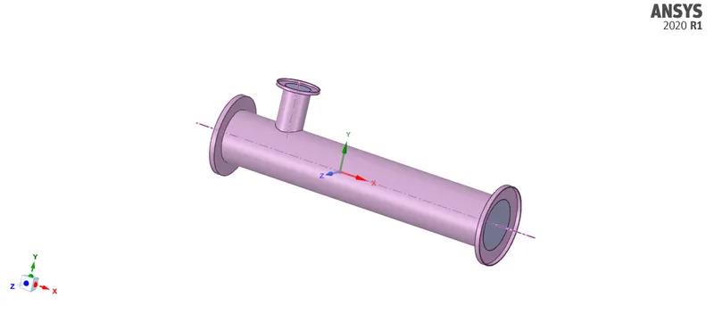
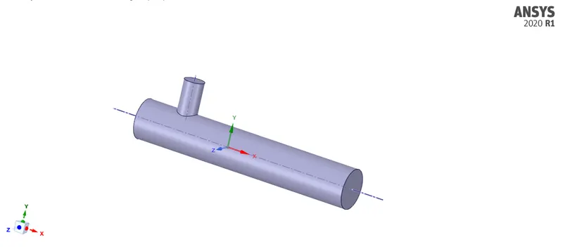
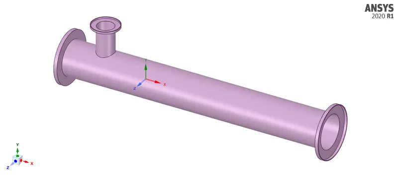
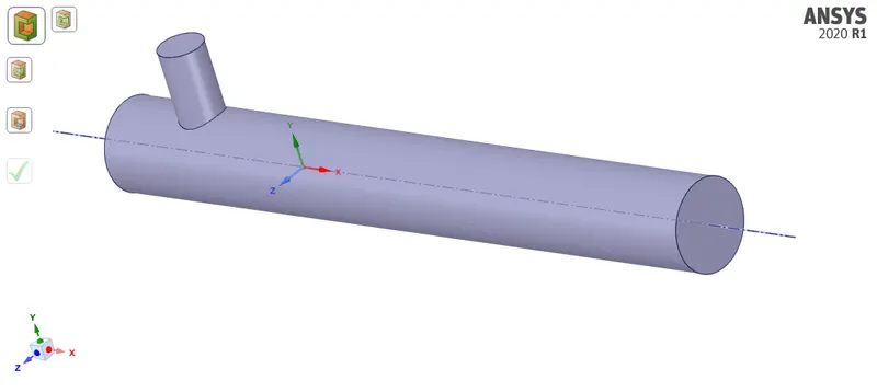
Create a project for the current study in the Ansys workbench and save it. Then, the SpaceClaim window is opened. The geometry for both long and short pipes is created in SpaceClaim. The wet volume needed for the simulation is extracted using the edge selection method and the solid volume is suppressed.
Short pipe - Geometry:
Short pipe - Volume:
Long pipe - Geometry:
Long pipe - Volume:
MESH GENERATION:
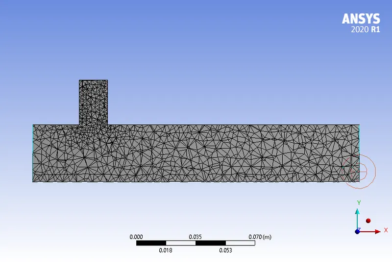
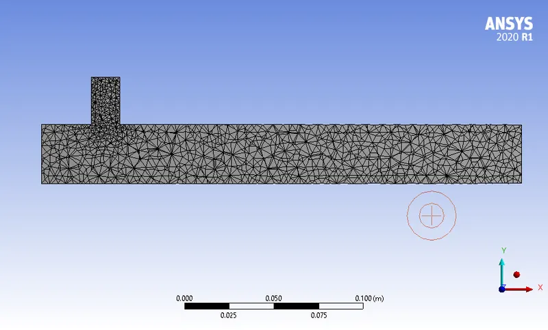
After the successful creation of geometry, the SpaceClaim window is closed and the meshing window is opened. the geometry will load automatically. Each face is named and the mesh is generated for a pre-set mesh size of 0.01.
Short pipe - Mesh:
Mesh size: 0.01
Cell count: 12760
Long pipe - Mesh:
Mesh size: 0.01
Cell count: 15689
CASE SETUP:
Once the mesh is generated, the fluent window is opened and the wet volume along with the mesh is loaded automatically. Initially, a mesh check is done. Then, the suitable boundary conditions are specified. For inlet passages, Velocity-inlet BC is used. For outlet, Pressure-outlet BC is used. A steady-state pressure-based solver with absolute velocity is used since it is a low Mach number flow. K-`epsilon` realizable turbulence model is chosen. Report definitions for the Area-weighted average plot and the standard deviation plot for mixing temperature at the outlet are created.
SOLUTION:
The solution is initialized using the hybrid initialization method. Then, the number of iterations is specified and the calculation is run until convergence is obtained. If the solution doesn't converge, then the number of iterations has to be increased until the solution converges. The Residuals, Area-weighted average of outlet temperature, and standard deviation of outlet temperature plots are obtained and the fluent window is closed. The work is saved automatically. Then the CFD-Post is opened for post-processing. From the CFD-Post, temperature, and velocity contours can be obtained by creating a plane along and across the pipe. Line-plots for temperature and velocity are obtained by creating a line along and across the pipe.
MESH SENSITIVITY ANALYSIS:
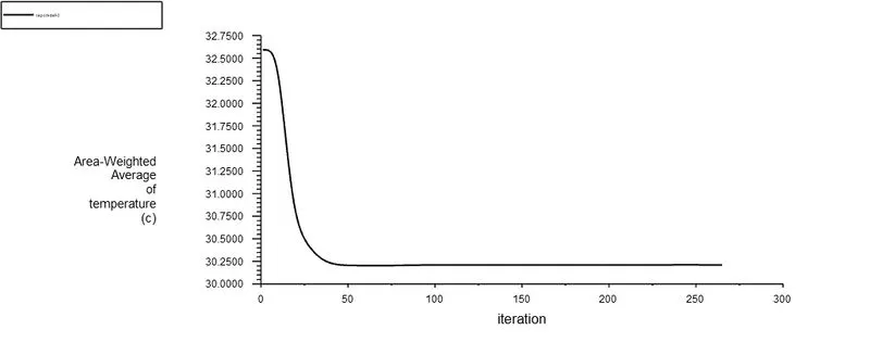
Mesh sensitivity analysis is performed to declare that the simulation is not a function of mesh points i.e., varying the number of mesh points should not affect the results of the simulation under study. In this study, the mesh size is varied as 0.01 and 0.005 for case 1a (short pipe with MR=2), and the simulations are run.
| MESH SIZE - 0.01 | MESH SIZE - 0.005 | |
| MESH COUNT | 12760 | 14330 |
| ITERATIONS | 265 | 400 |
| NUMERICAL `T_(avg)` | `30.25^oC` | `30.25^oC` |
| EXACT `T_(avg)` | `30.44^oC` | `30.44^oC` |
Mesh size - 0.01:
Mesh size - 0.005:
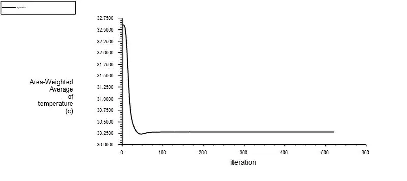
- In both these cases, the outlet temperature is not the same as that of the exact value but close to it.
- It is observed that with an increase in the mesh count by decreasing the mesh size, the outlet temperature remains the same.
- With an increase in the mesh count, the number of iterations is increased. In order to minimize the computational time, a mesh size of 0.01 is chosen for all the cases.
RESULTS AND DISCUSSIONS:
Residuals:
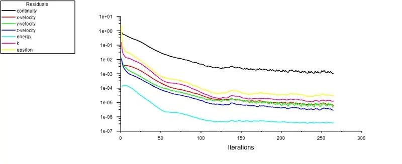
Case 1a: A short pipe with MR=2
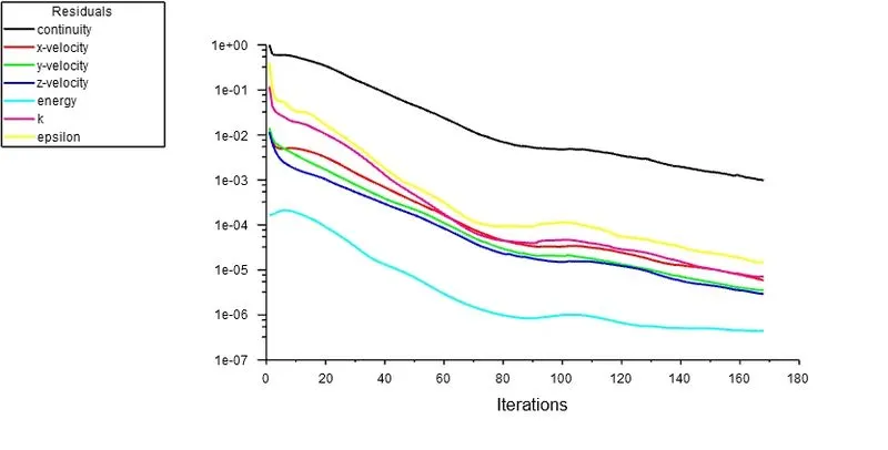
Case 1b: A short pipe with MR=4
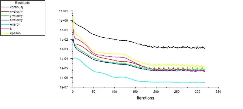
Case 2a: A long pipe with MR=2
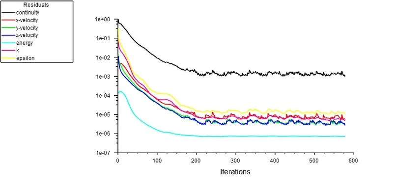
Case 2b: A long pipe with MR=4
Discussions:
Convergence is declared when the residuals attain a constant value or a constant pattern. The number of iterations in each case are as follows:
Case 1a: Short pipe with MR=2 `->` 265
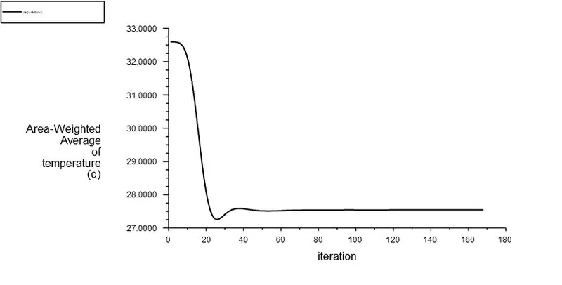
Case 1b: Short pipe with MR=4 `->` 168
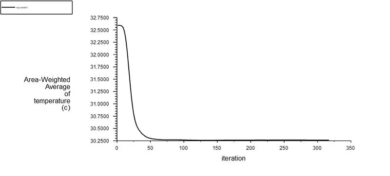
Case 2a: Long pipe with MR=2 `->` 317
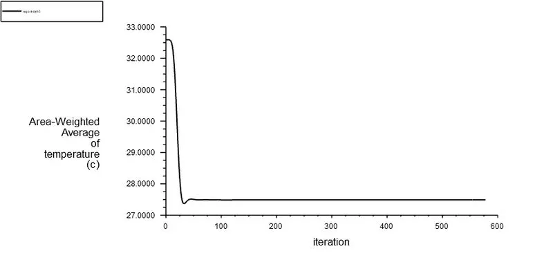
Case 2b: Long pipe with MR=4 `->` 578
Area-weighted average of temperature at outlet:
Case 1a: A short pipe with MR=2
Case 1b: A short pipe with MR=4
Case 2a: A long pipe with MR=2
Case 2b: A long pipe with MR=4
Discussions:
| CASE 1A | CASE 1B | CASE 2A | CASE 2B | |
| NUMERICAL VALUE | `30.25^oC` | `27.5^oC` | `30.25^oC` | `27.5^oC` |
| EXACT VALUE | `30.44^oC` | `27.63^oC` | `30.44^oC` | `27.63^oC` |
- The numerical values are closer to the exact values in all four cases.
- The temperature at the outlet decreases with an increase in the momentum ratio for both short and long pipe.
Standard deviation of temperature at outlet:
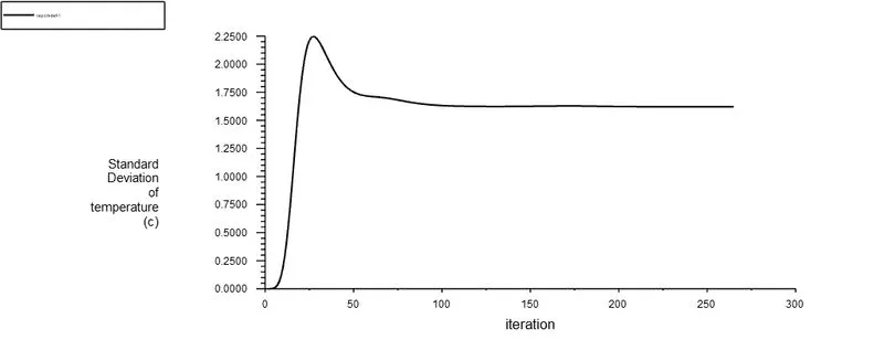
Case 1a: A short pipe with MR=2
Case 1b: A short pipe with MR=4
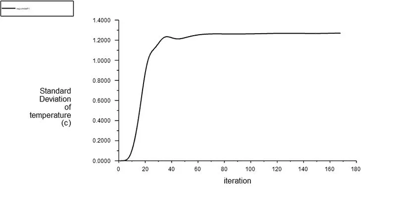
Case 2a: A long pipe with MR=2
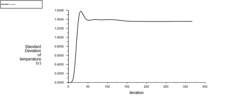
Case 2b: A long pipe with MR=4
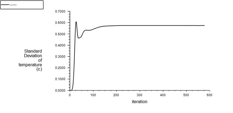
Discussions:
| CASE 1A | CASE 1B | CASE 2A | CASE 2B | |
| MOMENTUM RATIO | 2 | 4 | 2 | 4 |
| STANDARD DEVIATION OF TEMPERATURE AT OUTLET (`IN ^o C`) |
1.75 |
1.2 | 1.4 | 0.55 |
- The standard deviation is an indication of mixing effectiveness
- In all four cases, the standard deviation is in the range of `0.5^oC` - `1.75^oC` which is very low indicating effective mixing.
- For the same MR, the mixing effectiveness increases with an increase in pipe length.
- For the same pipe length, the mixing effectiveness increases with an increase in MR.
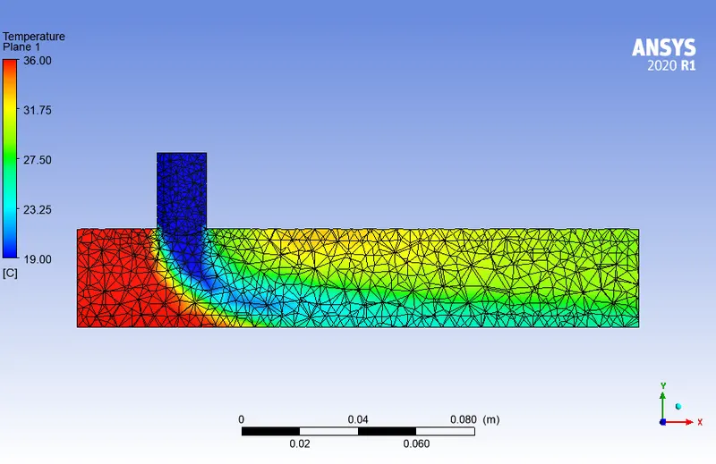
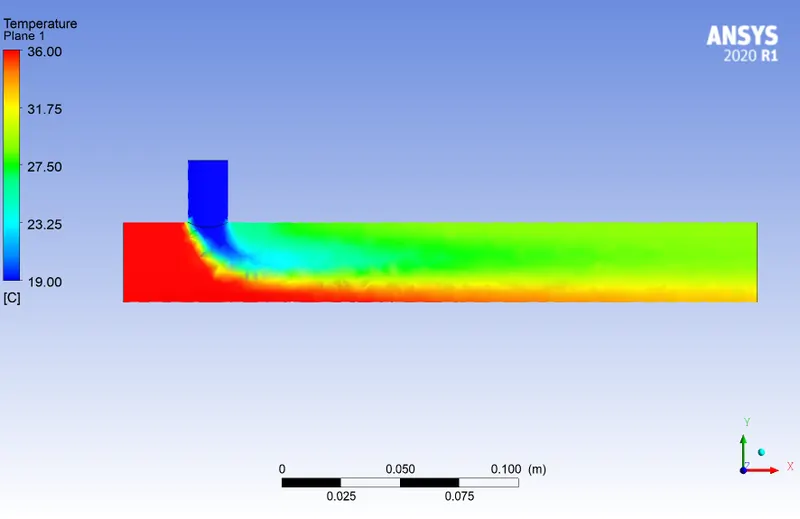
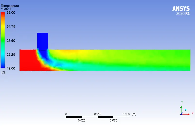
Temperature contours along the pipe:
Case 1a: A short pipe with MR=2
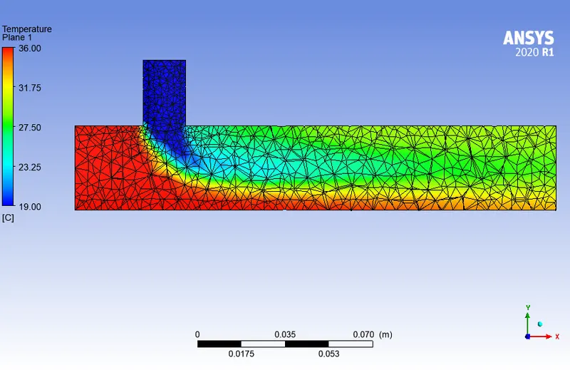
Case 1b: A short pipe with MR=4
Case 2a: A long pipe with MR=2
Case 2b: A long pipe with MR=4
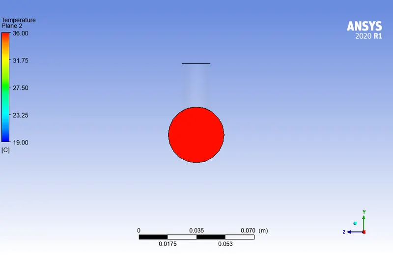
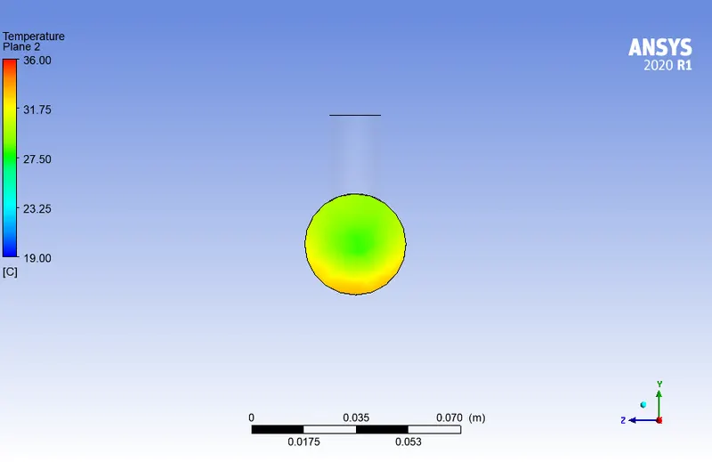
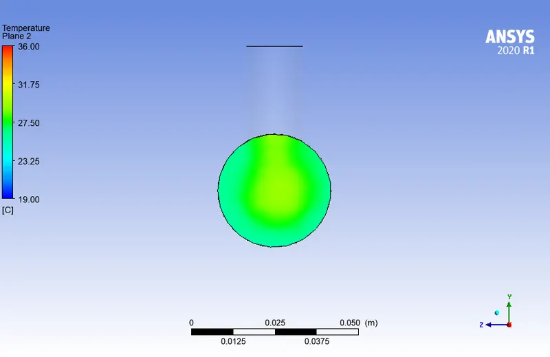
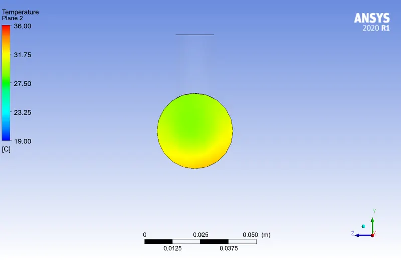
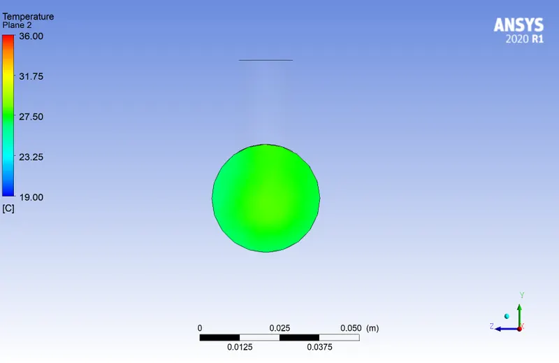
Temperature contours across the pipe:
Inlet:
Outlet:
Case 1a: A short pipe with MR=2
Case 1b: A short pipe with MR=4
Case 2a: A long pipe with MR=2
Case 2b: A long pipe with MR=4
Discussions:
- For short and long pipes, the mixing is more uniform with an increase in the MR.
- For the same MR, the outlet temperature has reduced significantly with an increase in the pipe length.
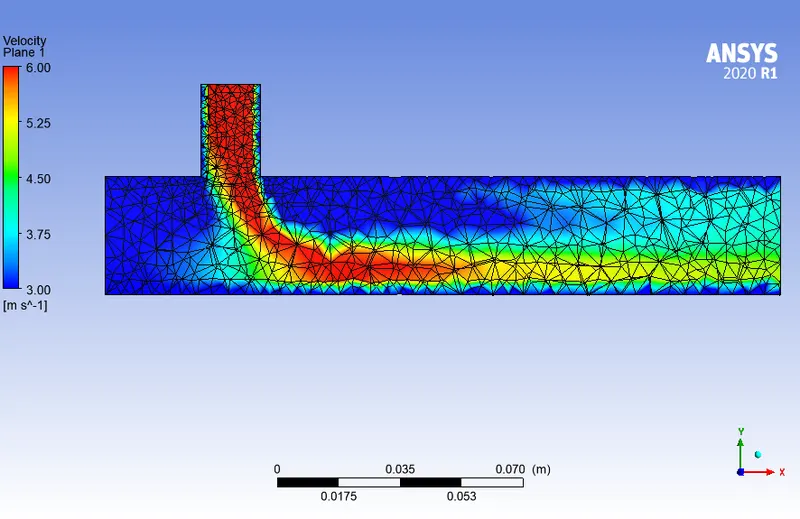
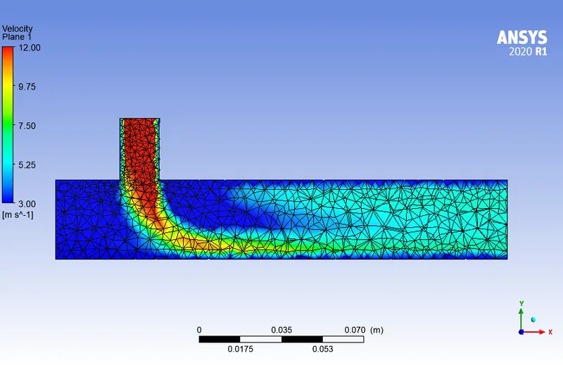
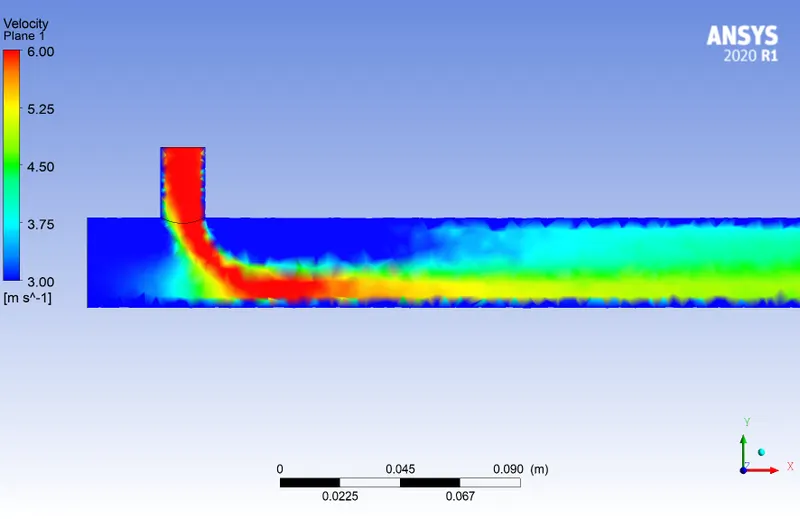
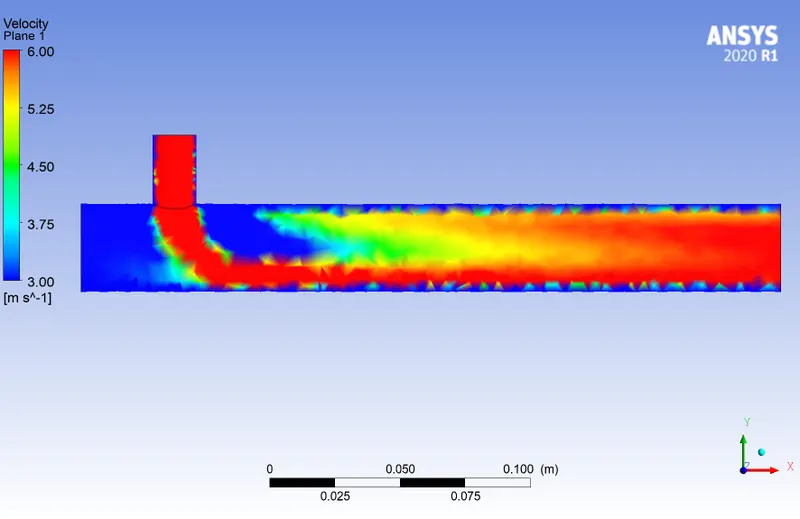
Velocity contours along the pipe:
Case 1a: A short pipe with MR=2
Case 1b: A short pipe with MR=4
Case 2a: A long pipe with MR=2
Case 2b: A long pipe with MR=4
Velocity contours across the pipe:
Inlet:
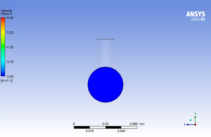
Outlet:
Case 1a: A short pipe with MR=2
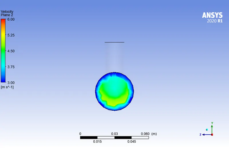
Case 1b: A short pipe with MR=4
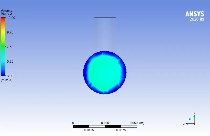
Case 2a: A long pipe with MR=2
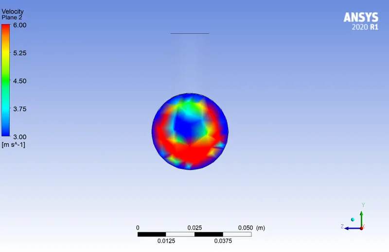
Case 2b: A long pipe with MR=4
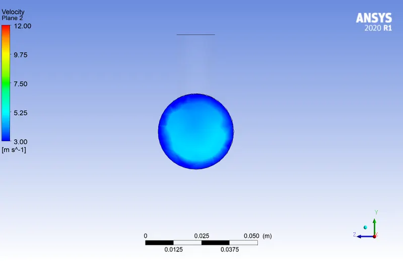
Discussions:
- With an increase in the MR, there is an increase in the velocity at the outlet.
- Also, with an increase in the MR, the velocity distribution is more uniform at the outlet.
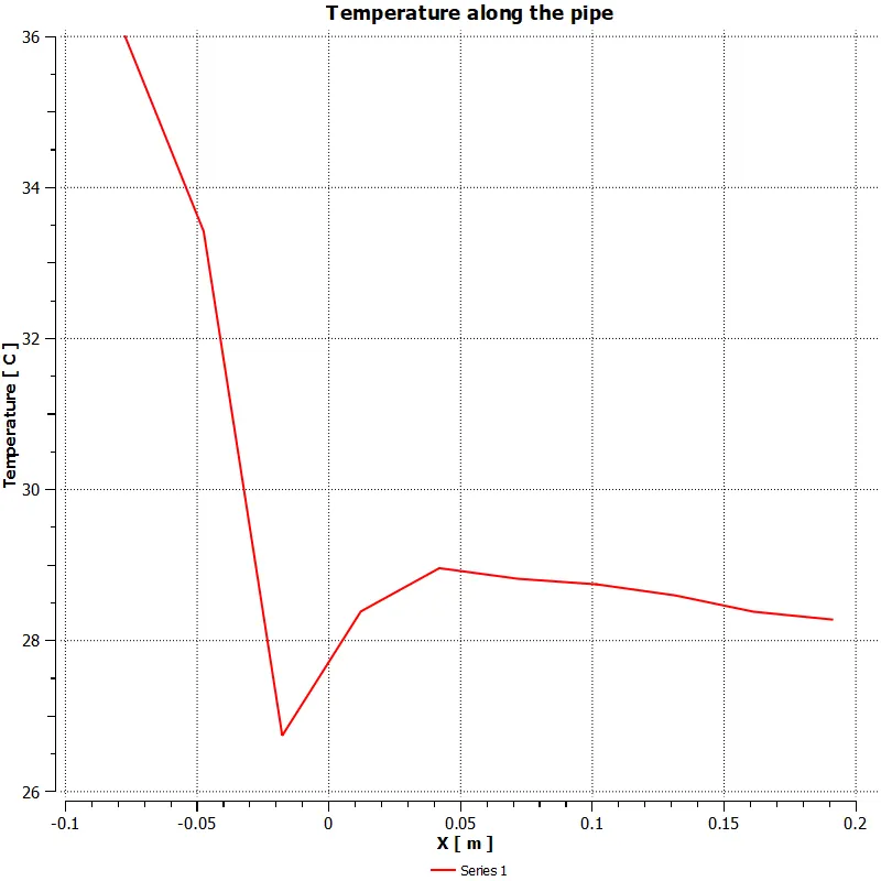
Line-plots of temperature along the pipe:
Case 1a: A short pipe with MR=2
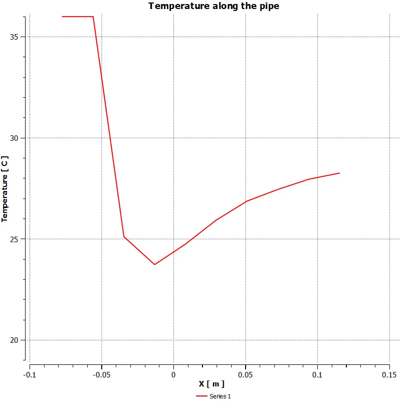
Case 1b: A short pipe with MR=4
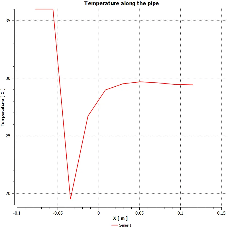
Case 2a: A long pipe with MR=2
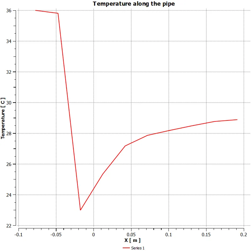
Case 2b: A long pipe with MR=4
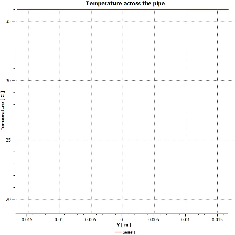
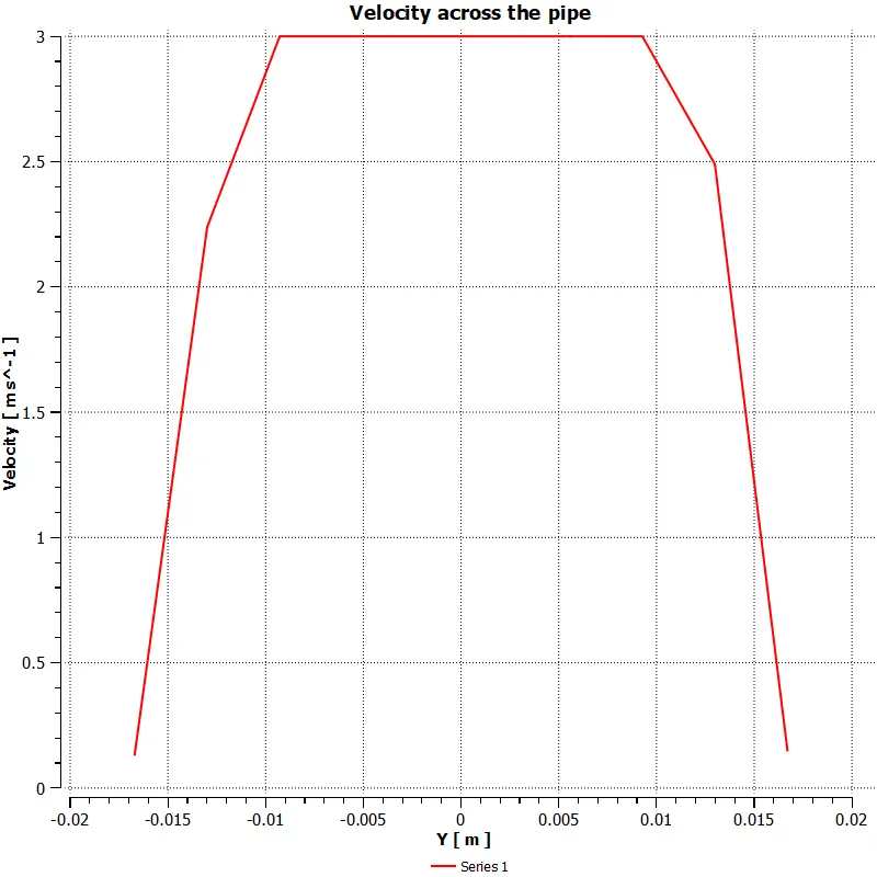
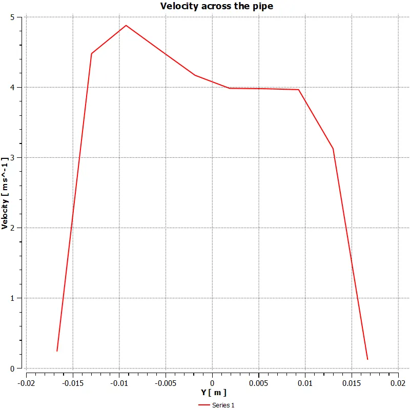
Line-plots of temperature across the pipe:
Inlet:
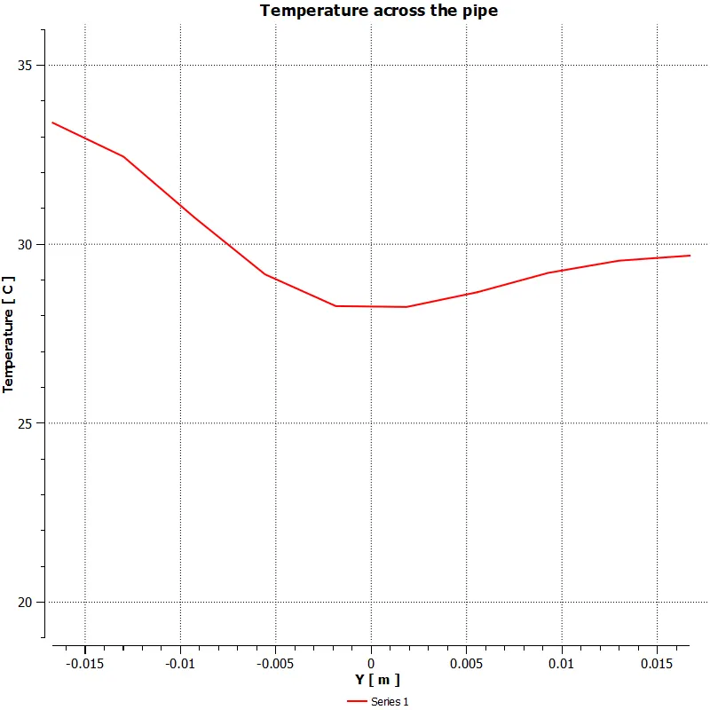
Outlet:
Case 1a: A short pipe with MR=2
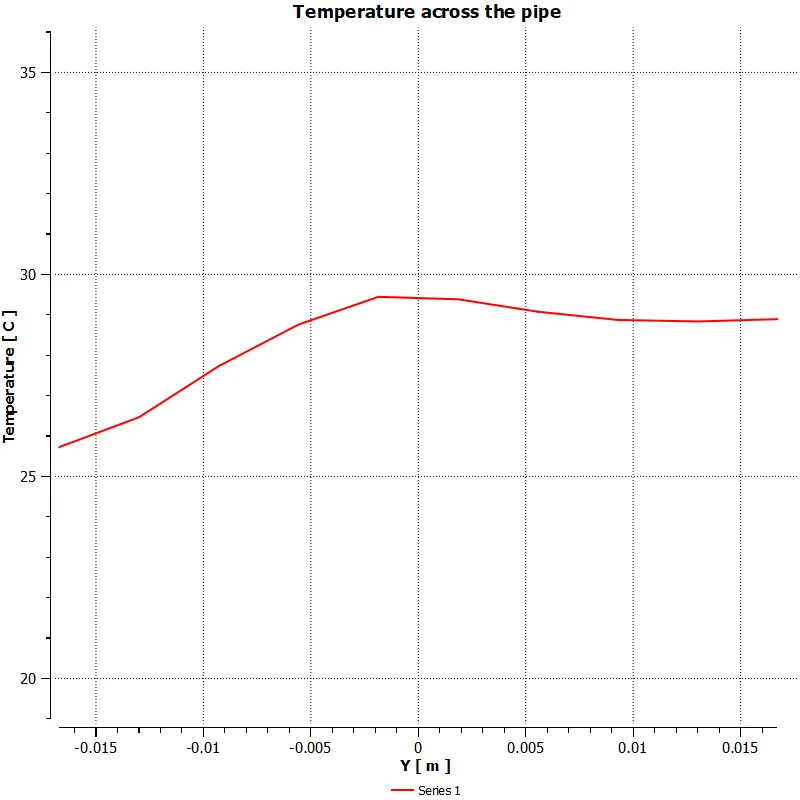
Case 1b: A short pipe with MR=4
Case 2a: A long pipe with MR=2
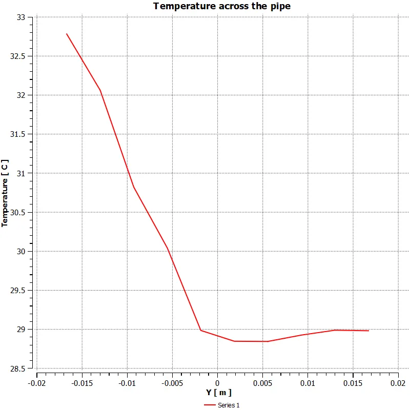
Case 2b: A long pipe with MR=4
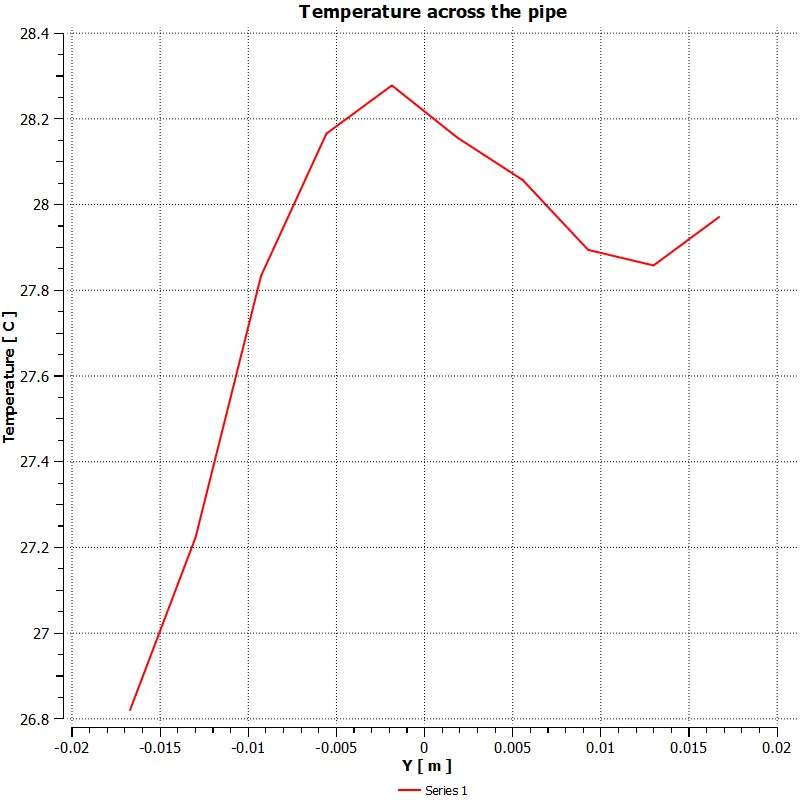
Discussions:
- Along the pipe, due to the hot inlet air, the temperature is high initially and then sees a dip due to the cold inlet airflow. Finally, the temperature reaches an optimum value.
- Across the pipe, the temperature is low at the top portion for low MR and the bottom portion for high MR.
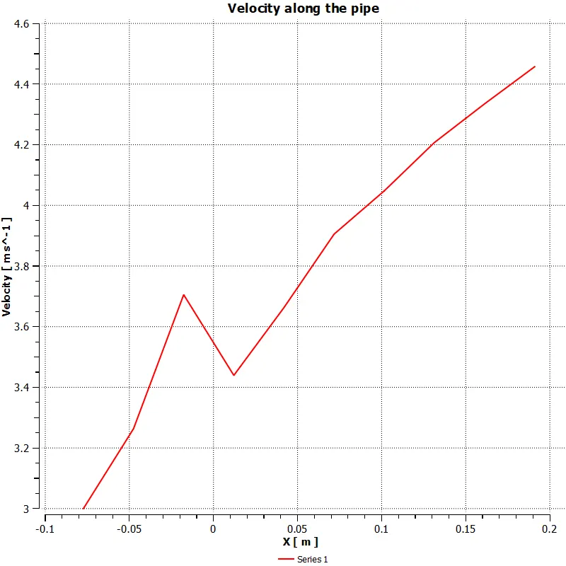
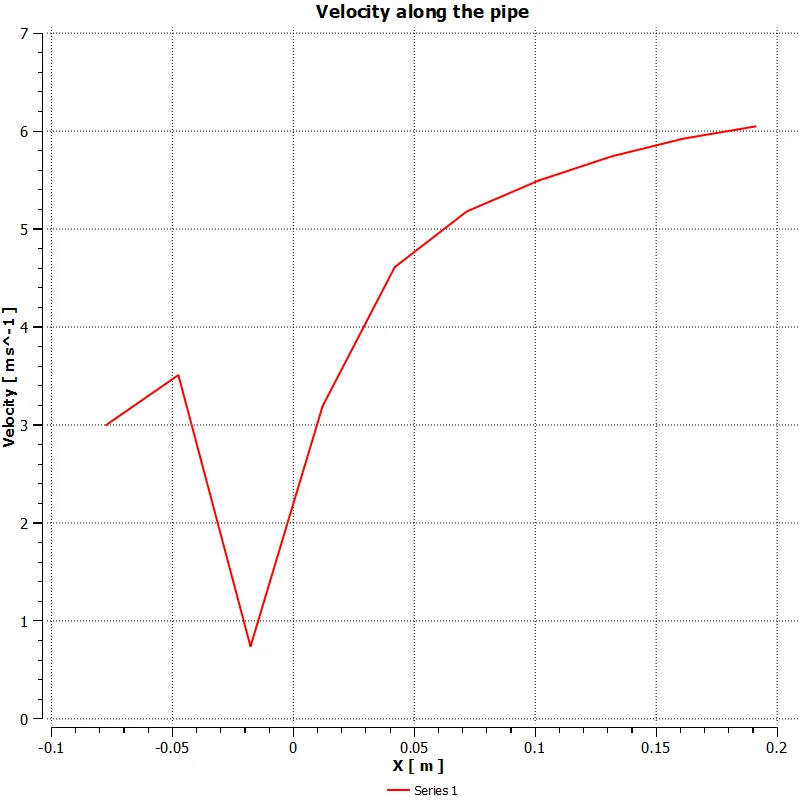
Line-plots of velocity along the pipe:
Case 1a: A short pipe with MR=2
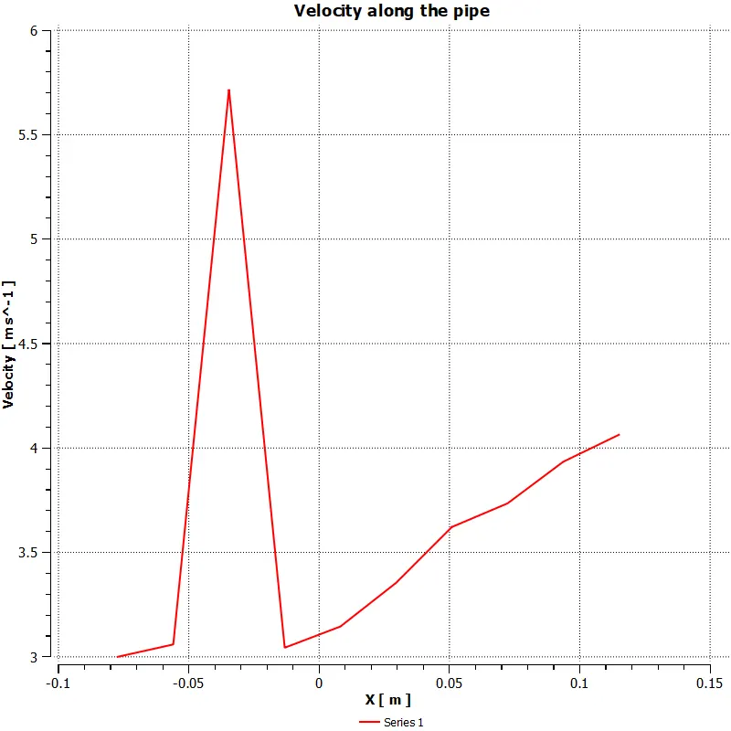
Case 1b: A short pipe with MR=4
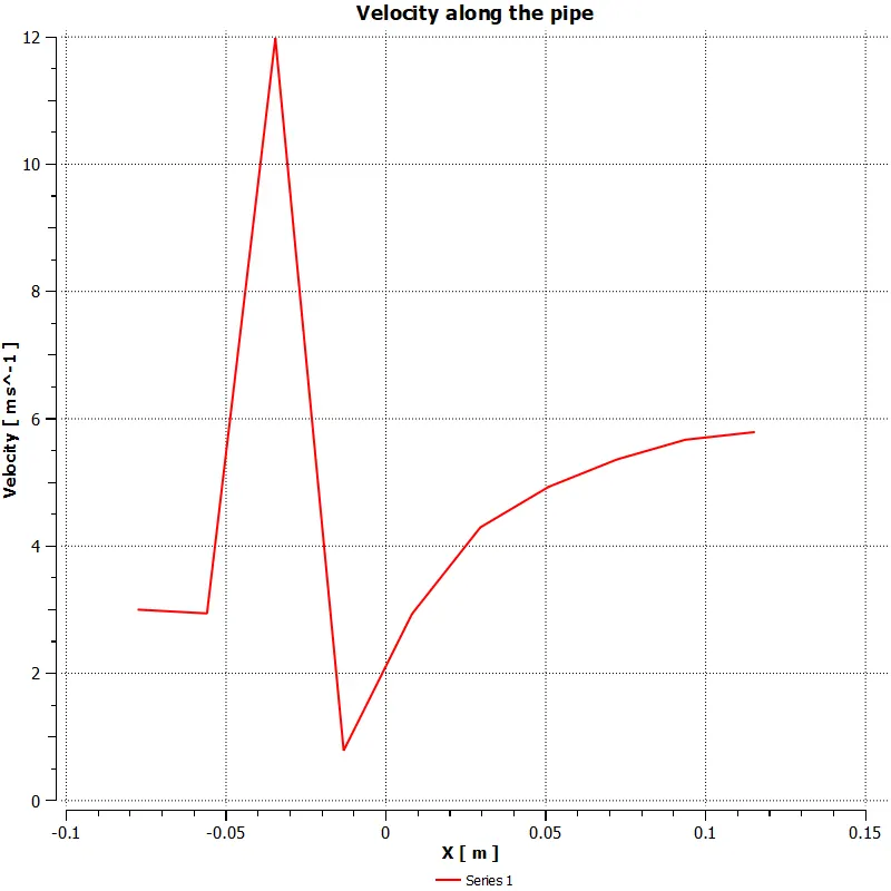
Case 2a: A long pipe with MR=2
Case 2b: A long pipe with MR=4
Line-plots of velocity across the pipe:
Inlet:
Outlet:
Case 1a: A short pipe with MR=2
Case 1b: A short pipe with MR=4
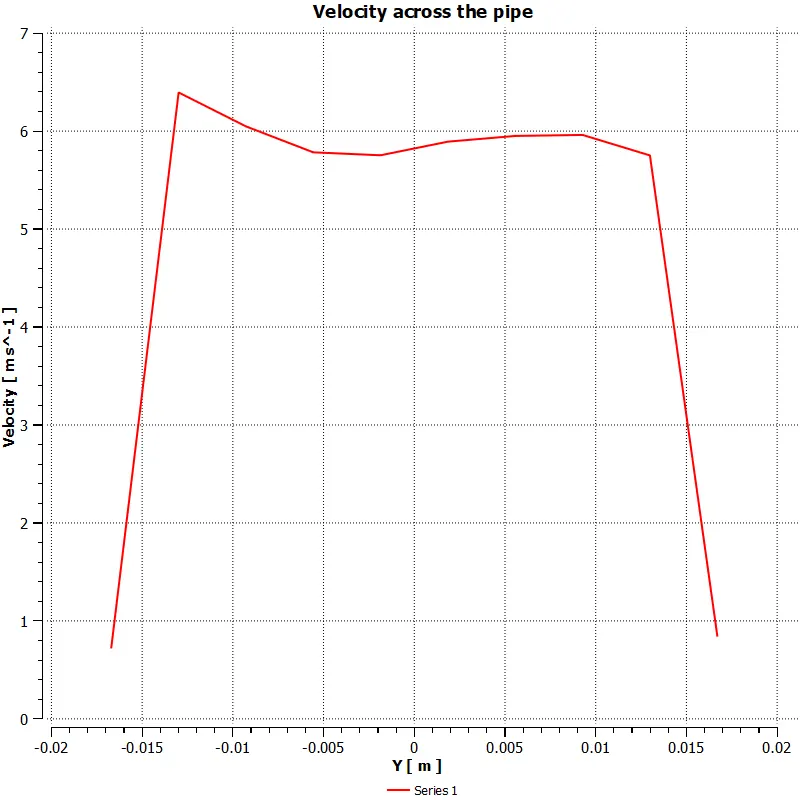
Case 2a: A long pipe with MR=2
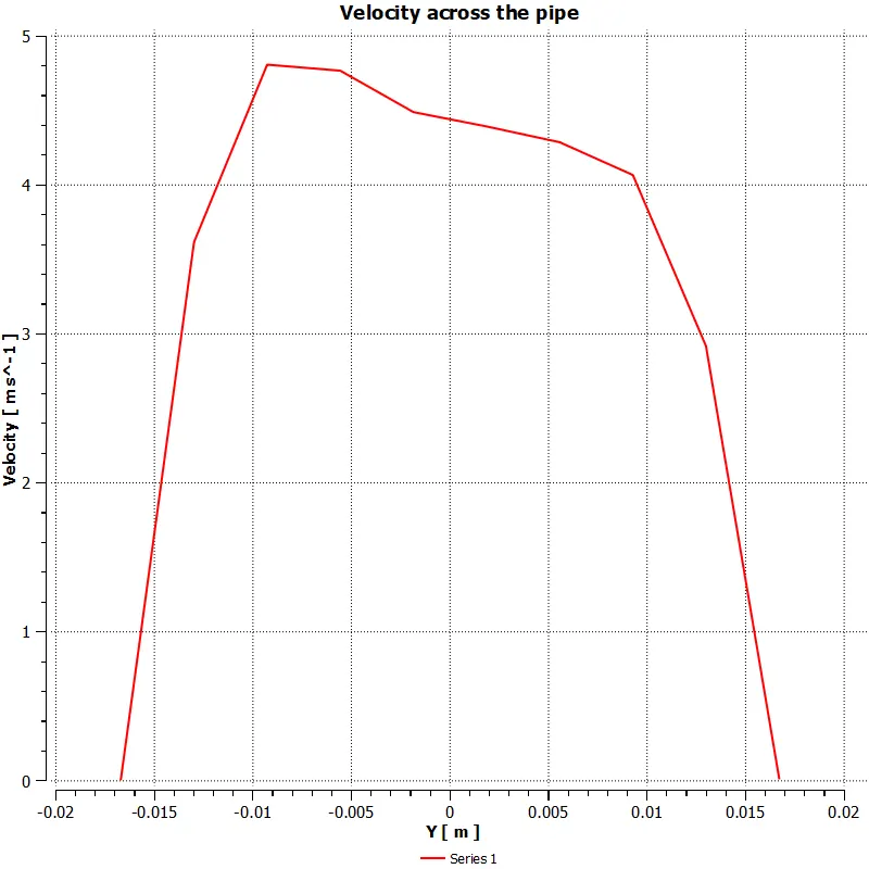
Case 2b: A long pipe with MR=4
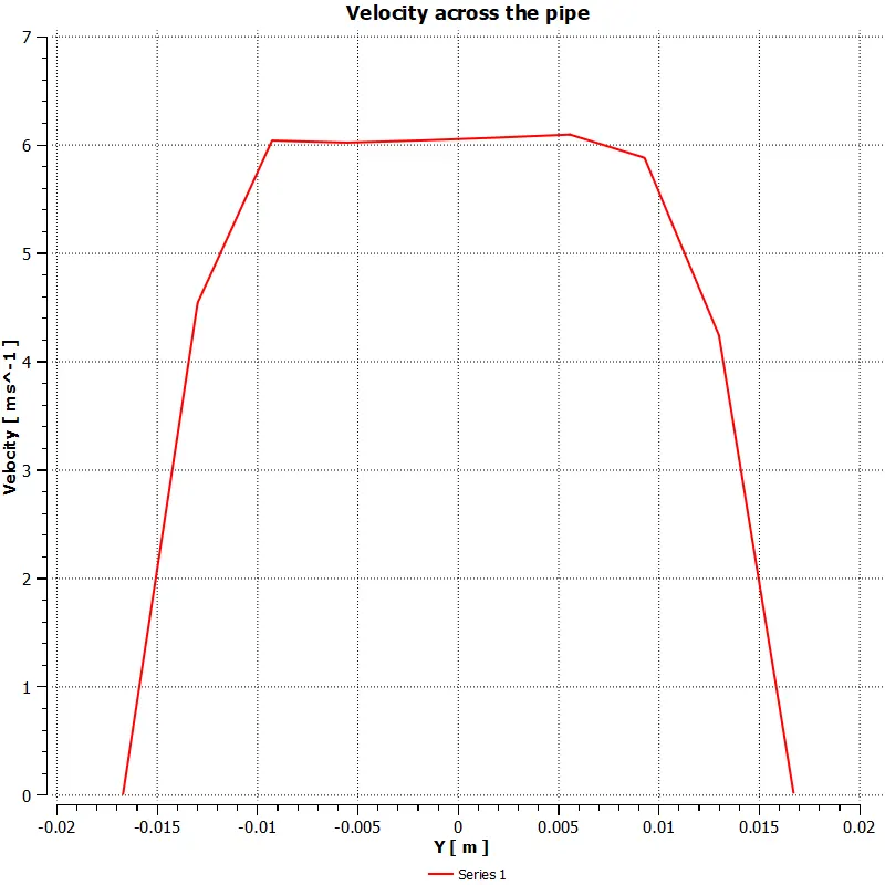
Discussions:
- Along the pipe, the velocity is low at the starting end and increases as the cold air enter and then attains an average value.
- Across the pipe, with an increase in the MR, the velocity profile is more uniform at the outlet.
CONCLUSIONS:
- The mixing effectiveness increases with an increase in the pipe length for the same momentum ratio because more time is available for the air streams to mix in a long pipe than a short one.
- The mixing effectiveness increases with an increase in the momentum ratio for the same pipe length because with an increased cold air velocity the mass flow rate of cold air is increased resulting in better mixing.