Week 4 - CHT Analysis on Exhaust port
CHT ANALYSIS ON EXHAUST PORT
Introduction:
Conjugate heat transfer corresponds with the combination of heat transfer in solids and heat transfer in fluids. Conjugate heat transfer is observed in many situations. For example, heat sinks are optimized to combine heat transfer by conduction in the heat sink with the convection in the surrounding fluid. The Conjugate Heat Transfer (CHT) analysis type allows for the simulation of heat transfer between solid and fluid domains by exchanging thermal energy at the interfaces between them. Typical applications of this analysis type exist as, but are not limited to, the simulation of heat exchangers, cooling of electronic equipment, and general-purpose cooling and heating systems.
Baseline simulation:
1. Geometry:
A CAD model of the exhaust manifold is imported into spaceclaim.
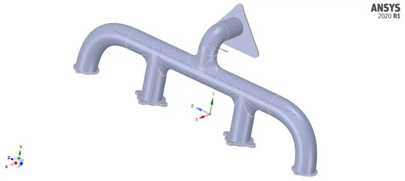
The next step is to extract the fluid volume. This is done by using the prepare option, edge selection has opted and the fluid volume is extracted.
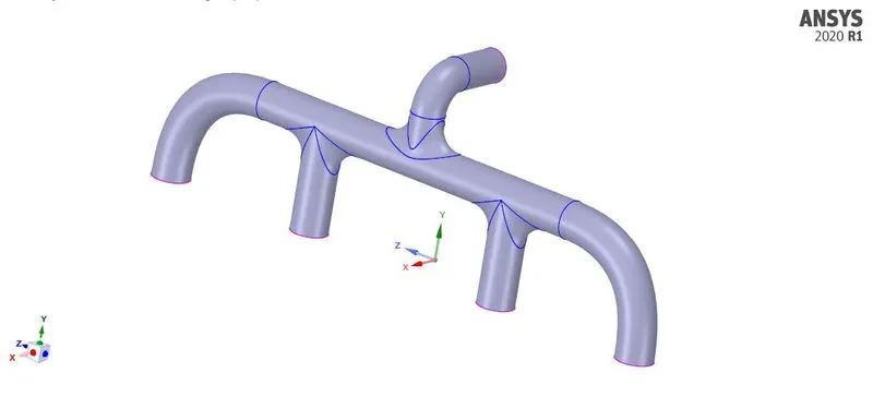
There are interfaces or surfaces where the fluid volume and the solid share. This should be made to share or enabled to share using the share prep option in the workbench.
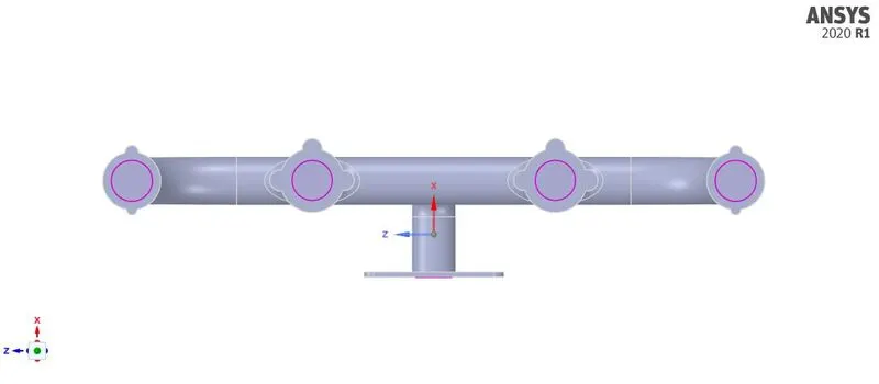
The solid and fluid volume components are selected and moved to a new component and named final geometry. Shared topology is enabled.
2. Meshing:
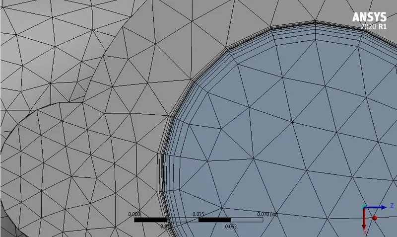
Since it is a baseline simulation, the default meshing that Ansys mesher does is checked. Named selections are provided to all the parts to apply boundary conditions when physics is set up. There are three named selections - (i) inlets, from where the hot exhaust gases enter the exhaust manifold, (ii) outlet, from where the exhaust gases leave, and (iii) outer wall convection.
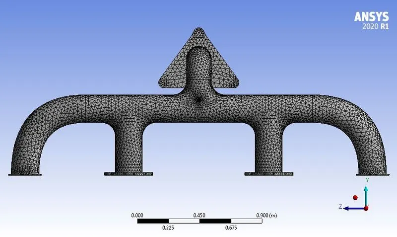
Mesh metrics:
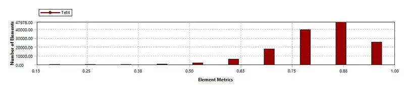
3. Solution:
Physics:
The materials assigned for the fluid and solid are air and aluminium respectively.
Properties of air and aluminium:
Air:
| Density | 1.225 kg/`m^3` |
| `C_p` | 1006.43 J/kg K |
| Thermal conductivity | 0.0242 W/m K |
| Viscosity | 1.7894e-5 kg/m s |
Aluminium:
| Density | 2719 kg/`m^3` |
| `C_p` | 871 J/kg K |
| Thermal conductivity | 0.0242 W/m K |
A pressure-based solver is used. Velocity formulation is absolute and perpendicular to the boundary. Steady-state analysis is performed. Since the study is dealt with in horizontal condition, no gravity is turned on. The SIMPLE scheme is selected for the pressure-velocity coupling.
Boundary conditions:
- Inlets: For the inlets, the velocity of the fluid inflow is taken as 5 m/s and the temperature of the fluid is taken as 700 K.
- The outer wall is considered a convection wall with a heat transfer coefficient of 20 W/`m^2` K.
- Outlet: Pressure boundary condition
Hybrid initialisation is done. The simulation is run for 300 iterations.
4. Results:
Residuals plot:
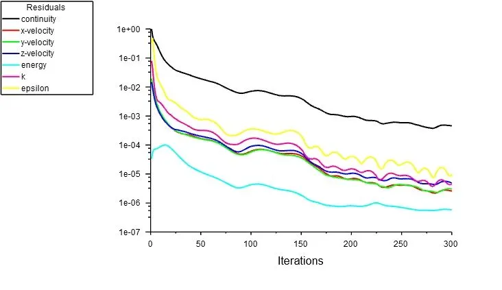
Temperature contour:
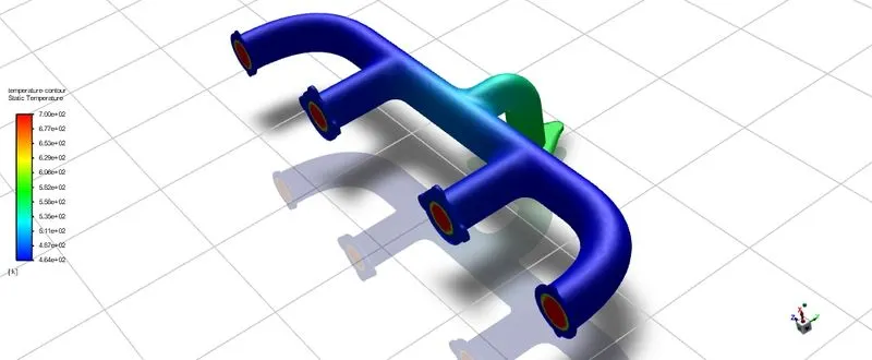
Velocity contour:
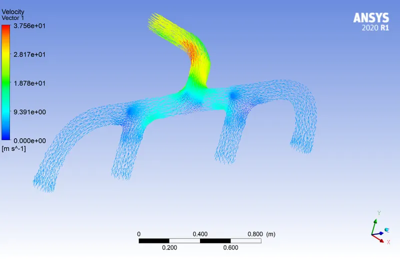
Wall heat transfer coefficient contour:
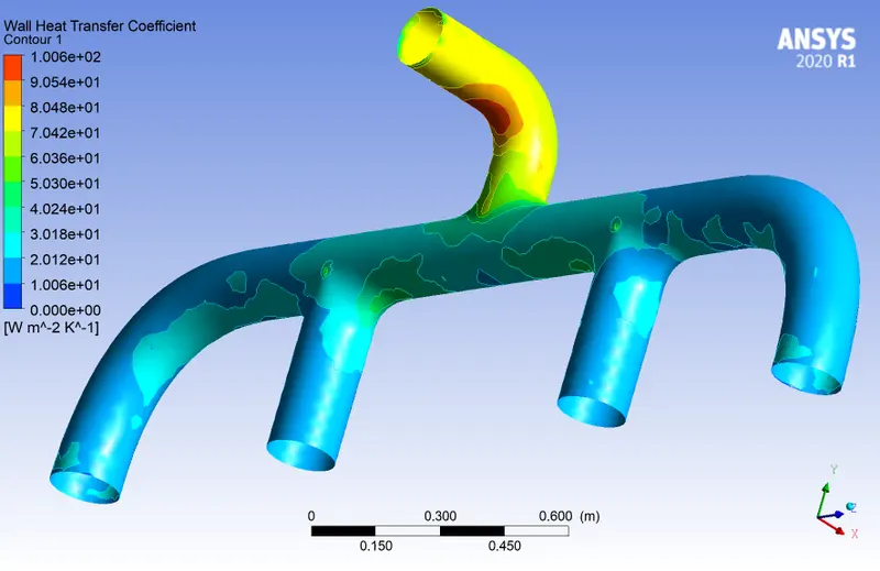
The baseline simulation gave coarse mesh results. Since the wall heat transfer coefficient is a wall phenomenon, wall modelling is required to capture the physics properly.
Refined case - 1:
In this study, the standard k-`epsilon` turbulence model is used. For standard k-`epsilon`, Y+ value should be in the range of 30 - 300. In case 1, the Y+ value chosen is 30.
Reynolds number:
Re = `(rho U L)/mu`
where,
`rho` = density of the fluid (kg/`m^3`)
U = Velocity of the incoming fluid (m/s)
D = Characteristic dimension of the geometry (m)
`mu` = Viscosity of the fluid (kg/m s)
For the present analysis:
`rho` = 1.225 kg/`m^3`
U = 5 m/s
D = inlet inner diameter = 0.1661 m
`mu` = 1.7894e-5 kg/m s
Re=`(1.225 * 5 * 0.1661)/(1.7894e-5)`
= 5.6854e+4
Skin friction coefficient:
`C_f` = `0.079 * Re^(-0.25)`
= `0.079 * (5.6854e+4)^(-0.25)`
= 0.0051
Wall shear stress:
`tau_w` = `(1/2) * C_f * rho * U^2`
= `(1/2) * 0.0051 * 1.225 * 5^2`
= 0.078
Friction velocity:
`U_f` = `(tau_w/rho)^0.5`
= `(0.078/1.225)^0.5`
0.2523
First layer thickness:
y = `(Y+ * mu)/(rho * U_f)`
= `(30 * 1.7894e-5)/(1.225 * 0.2523)`
= 1.7369 mm
Number of layers = 5
Growth rate GR = 1.2
Total thickness `T_t` = `y * (GR)^(n-1)`
= `1.7369 * (1.2)^(n-1)`
=3.6016 mm
Inflation layers are added to model the Y+ value.
Wall Y+ plot Vs position:
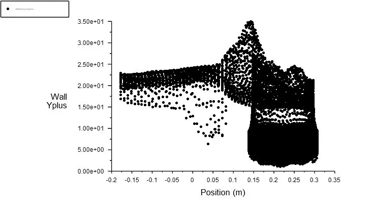
The wall Y+ value is not within the range of 30 - 300. Therefore this case is invalid. Now let's assume a Y+ plus value of 150 and observe the changes.
Refined case - 2:
In this study, the standard k-`epsilon` turbulence model is used. For standard k-`epsilon`, Y+ value should be in the range of 30 - 300. In case 1, the Y+ value chosen is 30.
Reynolds number:
Re = `(rho U L)/mu`
Re=`(1.225 * 5 * 0.1661)/(1.7894e-5)`
= 5.6854e+4
Skin friction coefficient:
`C_f` = `0.079 * Re^(-0.25)`
= `0.079 * (5.6854e+4)^(-0.25)`
= 0.0051
Wall shear stress:
`tau_w` = `(1/2) * C_f * rho * U^2`
= `(1/2) * 0.0051 * 1.225 * 5^2`
= 0.078
Friction velocity:
`U_f` = `(tau_w/rho)^0.5`
= `(0.078/1.225)^0.5`
0.2523
First layer thickness:
y = `(Y+ * mu)/(rho * U_f)`
= `(150 * 1.7894e-5)/(1.225 * 0.2523)`
= 8.39733 mm
Number of layers = 5
Growth rate GR = 1.2
Total thickness `T_t` = `y * (GR)^(n-1)`
= `8.39733 * (1.2)^(n-1)`
= 17.4127 mm
Inflation layers are added to model the Y+ value.
Wall Y+ plot Vs position:
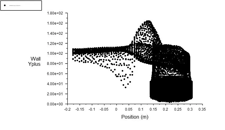
The maximum wall Y+ value is 160 which is within the range of 30 - 300. Therefore this case is valid.
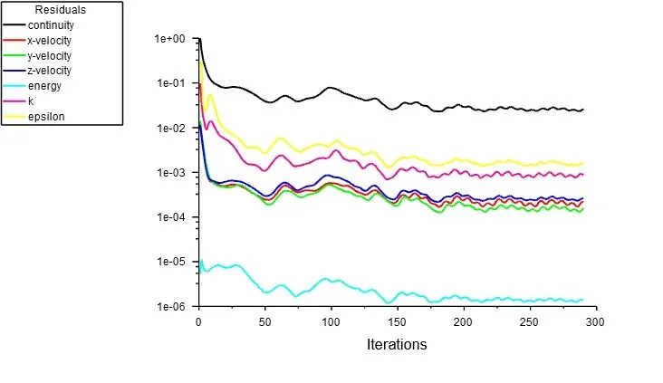
Residuals plot:
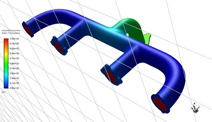
Temperature contour:
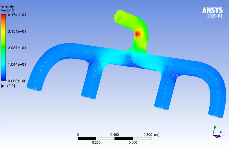
Velocity contour:
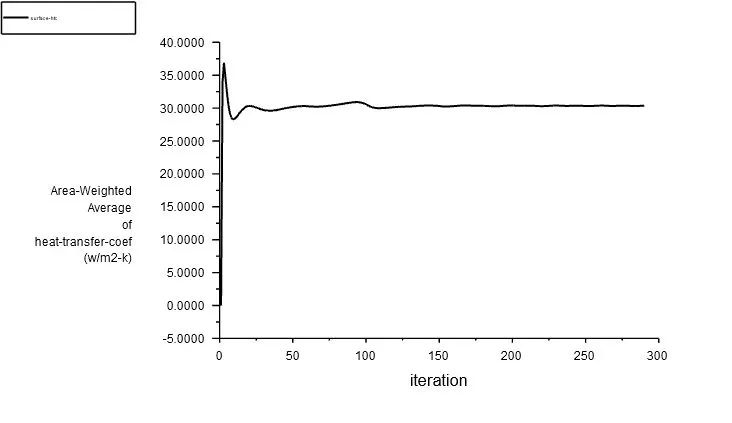
Surface heat transfer coefficient plot:
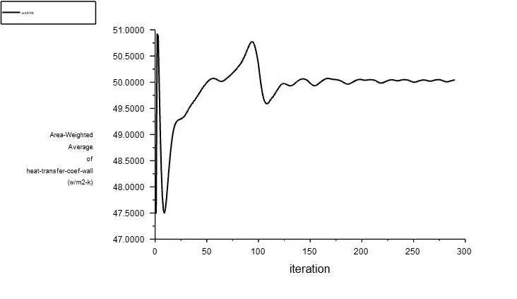
Wall heat transfer coefficient plot:
Difference between wall and surface heat transfer:
Assume that there is a layer that is very close to the wall. The wall heat transfer coefficient is higher than that of the upper layer.
Heat flux q = `h * (T_(fluid) - T_(wall))`
Since the wall temperature is higher, the temperature difference is less which makes the h value bigger.
Average value of surface htc = 30 W/`m^2` K
Average value of wall htc = 50 W/`m^2` K
Wall heat transfer coefficient contour:
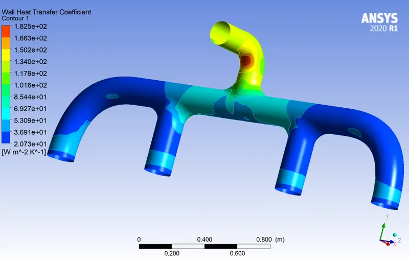
It is observed that the wall heat transfer coefficient is higher in the inner bend area which is coloured in red in the above contour. It is because of the fact that the velocity is high in this region. The reason for higher velocity is the pressure which reduces drastically near the outlet of the exhaust port and there is a sharp turn that reduces the pressure to a great extent. Due to high velocity, the mass flow rate is high in this region and so the wall heat transfer coefficient is also high because more heat will be transferred.
Validation:
Analytical solution:
Nusselt number Nu = `0.023 * Re^(0.8) * Pr^(0.3)`
Prandtl number Pr = `(mu * C_p)/k`
= `(1.7894e-5 * 1006.43)/0.0242`
= 0.74
Re = 5.6854e+4
Nu = `0.023 * (5.6854e+4)^(0.8) * 0.74^(0.3)`
= 133.75
Nu = `(h * D)/k`
h = `(Nu * k)/D`
= `(133.75 * 0.0242)/0.1661`
= 19.49 W/`m^2`K
Numerical solution:
Area weighted average of wall heat transfer coefficient from the refined case is 50 W/`m^2` K.
Wall heat transfer coefficient = 50/2 = 25 W/`m^2` K
Error = 28%
Conclusions:
- Maintaining proper Y+ plus value (within the range of 30 - 300) by varying the total thickness of the inflation layer provides better results. The mesh is well refined and so the results are better.
- The Wall heat transfer coefficient is higher than the surface heat transfer coefficient.
- The numerical wall heat transfer coefficient is almost similar to the analytical value with an error of 28% which is acceptable.
- The accuracy of the prediction highly depends on the velocity of the flow, Reynolds number and Nusselt number.