Week 11 - Simulation of Flow through a pipe in OpenFoam
SIMULATION OF FLOW THROUGH A PIPE IN OPENFOAM
Objectives:
- To write a program in Matlab/Octave that can generate the computational mesh automatically for any wedge angle and grading schemes.
- To validate the numerical solution with the Hagen-Poiseuille's equation.
Hagen-Poiseuille flow:
Hagen-Poiseuille flow (or simply Poiseuille flow) represents the flow through a circular pipe which is applicable to a variety of applications ranging from macroscopic pipes in industries to the flow of blood in the veins.
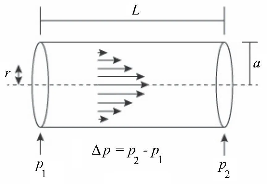
Hagen-Poiseuille's equation is a physical law that gives the pressure drop in an incompressible and laminar flow of a Newtonian fluid flowing through a long cylindrical pipe of constant cross-section.
- Average velocity `V_(avg) = (Re * mu)/(rho*D)`
- Maximum velocity `V_(max) = 2 * V_(avg)`
- Pressure drop `Deltap = (8*mu*L_(fdr)*V_(avg))/(r^2)`
- Kinematic pressure drop `Deltap_k = (Deltap)/rho`
- Wall shear stress `tau = (f/4)*((rho*V_(avg)^2)/2)`
where,
Re `->` Reynold's number `(rho*V_(avg)*D)/mu`
`mu` `->` Dynamic viscosity (`(N s)/m^2`)
`rho` `->` Density (`(kg)/m^3`)
D `->` Diameter of the pipe (m)
`L_(fdr)` `->` Length of the fully-developed region (m)
f `->` Darcy's friction factor (`64/(Re)`)
Hydrodynamic entry length:
It refers to the distance traveled by the flow after entering the pipe before it becomes fully developed.
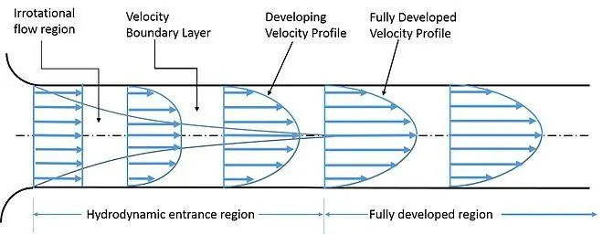
Awareness of entry length is necessary for the effective placement of the instrumentation such as flow meters. Hydrodynamic entry length for a laminar flow is given as:
`L_e` = 0.05 * Re * D
`L_(fdr) = L - L_e`
Geometry:
A circular pipe of diameter 0.02 m and length 3 m is considered for this challenge.
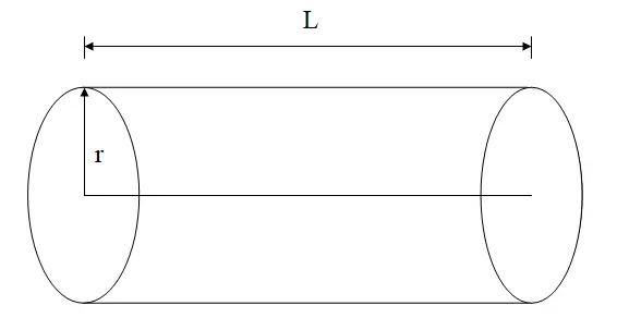
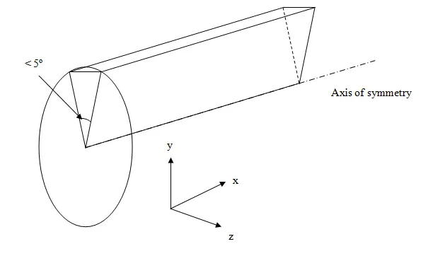
Geometry, loadings, boundary conditions, and materials are symmetric with respect to the x-axis. Therefore to decrease the computational effort and by taking advantage of the axis-symmetrical model, a reduced wedge model with a suitable wedge angle (<`5^o`) can be considered instead of a complete circular pipe for the simulation.
Preliminary data:
Diameter D = 0.02 m
Radius r = D/2 = 0.01 m
Total length L = 3 m
Reynold's number Re = 2100 (for laminar flow through a circular pipe)
Hydraulic entry length `L_e` = 0.05 * 2100 * 0.02 = 2.1 m
Length of the fully developed region `L_(fdr)` = L - `L_e` = 3 - 2.1 = 0.9 m
Wedge angle `theta` = `4^@`
Density `rho` = 998 kg/`m^3` (for water @ `20^@ C`)
Dynamic viscosity `mu` = 1e-03 `N s`/`m^2` (for water @ `20^@ C`)
Kinematic viscosity `nu` = `mu`/`rho` = 1e-06 `m^2`/s (for water @ `20^@ C`)
Matlab code - To generate blockMeshDict file:
clear all
close all
clc

%Reynolds number
Re=2100;
%Diameter of the pipe
D=0.02;
%Total length of the pipe
L=3;
%Hydraullic entry length
L_e=0.05*Re*D;
%Length of the fully developed region
L_f=L-L_e;
%Radius of the pipe
r=D/2;
%Wedge angle
theta=4;
%Dynamic viscosity of water at 20degC
mu=1e-03;
%Density of water at 20degC
rho=998;

%Hagen-Poiseuille equation
%Average velocity
v_avg=(Re*mu)/(rho*D);
%Maximum velocity
v_max=2*(v_avg);
%Pressure drop
del_p=(8*mu*L_f*v_avg)/(r^2);
%Kinematic pressure drop
del_p_k=del_p/rho;
%Friction factor
f=64/Re;
%Wall shear stress
tau=(f/4)*((rho*(v_avg)^2)/2);

%To create blockMeshDict file
%Header section
header1='/*--------------------------------*- C++ -*----------------------------------*\';
header2='  =========                 |';
header3='  \\      /  F ield         | OpenFOAM: The Open Source CFD Toolbox';
header4='   \\    /   O peration     | Website:  https://openfoam.org';
header5='    \\  /    A nd           | Version:  8';
header6='     \\/     M anipulation  |';
header7='\*---------------------------------------------------------------------------*/';

f1=fopen('blockMeshDict','w');
fprintf(f1, '%s\n',header1);
fprintf(f1, '%s\n',header2);
fprintf(f1, '%s\n',header3);
fprintf(f1, '%s\n',header4);
fprintf(f1, '%s\n',header5);
fprintf(f1, '%s\n',header6);
fprintf(f1, '%s\n',header7);

fprintf(f1, 'FoamFile\n{\n');
fprintf(f1, '\t %s \t 2.0;\n','version');
fprintf(f1, '\t %s \t ascii;\n','format');
fprintf(f1, '\t %s \t\t dictionary;\n','class');
fprintf(f1, '\t %s \t blockMeshDict;\n','object');
fprintf(f1, '}\n');

header8='// * * * * * * * * * * * * * * * * * * * * * * * * * * * * * * * * * * * * * //';
fprintf(f1, '%s\n\n',header8);
fprintf(f1, 'convertToMeters 1;\n\n');

%Vertices section
fprintf(f1, 'vertices\n');
fprintf(f1, '(\n');
fprintf(f1, '\t (%d %d %d)\n',0,0,0);
fprintf(f1, '\t (%d %d %d)\n',0,r*cosd(theta/2),r*sind(theta/2));
fprintf(f1, '\t (%d %d %d)\n',0,r*cosd(theta/2),-r*sind(theta/2));
fprintf(f1, '\t (%d %d %d)\n',L,0,0);
fprintf(f1, '\t (%d %d %d)\n',L,r*cosd(theta/2),r*sind(theta/2));
fprintf(f1, '\t (%d %d %d)\n',L,r*cosd(theta/2),-r*sind(theta/2));
fprintf(f1, ');\n\n');

%Blocks section
fprintf(f1, 'blocks\n');
fprintf(f1, '(\n');
fprintf(f1, '\t hex (0 3 5 2 0 3 4 1) (%d %d %d)',500,25,1);
fprintf(f1, ' simpleGrading (1 0.2 1)\n\n');
fprintf(f1, ');\n\n');

%Edges section
fprintf(f1, 'edges\n');
fprintf(f1, '(\n');
fprintf(f1, '\t arc %d %d (%d %d %d)\n',1,2,0,r,0);
fprintf(f1, '\t arc %d %d (%d %d %d)\n',4,5,L,r,0);
fprintf(f1, ');\n\n');

%Boundary section
fprintf(f1, 'boundary\n');
fprintf(f1, '(\n');
%Inlet
fprintf(f1, '\t inlet \n');
fprintf(f1, '\t {\n');
fprintf(f1, '\t\t type patch;\n');
fprintf(f1, '\t\t faces \n');
fprintf(f1, '\t\t (\n');
fprintf(f1, '\t\t\t (0 1 2 0)\n');
fprintf(f1, '\t\t );\n');
fprintf(f1, '\t }\n');
%Outlet
fprintf(f1, '\t outlet \n');
fprintf(f1, '\t {\n');
fprintf(f1, '\t\t type patch;\n');
fprintf(f1, '\t\t faces \n');
fprintf(f1, '\t\t (\n');
fprintf(f1, '\t\t\t (3 5 4 3)\n');
fprintf(f1, '\t\t );\n');
fprintf(f1, '\t }\n');
%Top
fprintf(f1, '\t top \n');
fprintf(f1, '\t {\n');
fprintf(f1, '\t\t type wall;\n');
fprintf(f1, '\t\t faces \n');
fprintf(f1, '\t\t (\n');
fprintf(f1, '\t\t\t (1 4 5 2)\n');
fprintf(f1, '\t\t );\n');
fprintf(f1, '\t }\n');
%Front
fprintf(f1, '\t front \n');
fprintf(f1, '\t {\n');
fprintf(f1, '\t\t type wedge;\n');
fprintf(f1, '\t\t faces \n');
fprintf(f1, '\t\t (\n');
fprintf(f1, '\t\t\t (0 3 4 1)\n');
fprintf(f1, '\t\t );\n');
fprintf(f1, '\t }\n');
%Back
fprintf(f1, '\t back \n');
fprintf(f1, '\t {\n');
fprintf(f1, '\t\t type wedge;\n');
fprintf(f1, '\t\t faces \n');
fprintf(f1, '\t\t (\n');
fprintf(f1, '\t\t\t (0 2 5 3)\n');
fprintf(f1, '\t\t );\n');
fprintf(f1, '\t }\n');
%Axis
fprintf(f1, '\t axis \n');
fprintf(f1, '\t {\n');
fprintf(f1, '\t\t type empty;\n');
fprintf(f1, '\t\t faces \n');
fprintf(f1, '\t\t (\n');
fprintf(f1, '\t\t\t (0 3 3 0)\n');
fprintf(f1, '\t\t );\n');
fprintf(f1, '\t }\n');
fprintf(f1, ');\n\n');

%Final section
fprintf(f1, 'mergePatchPairs\n');
fprintf(f1, '(\n');
fprintf(f1, ');\n');

header9='// ************************************************************************* //';
fprintf(f1, '%s\n',header9);
fclose(f1);
Mesh specifications:
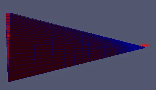
- Number of cells along the x-direction = 500
- Number of cells along the y-direction = 25
- Number of cells along the z-direction = 1
Simple grading factor:
- Along x-direction = 1
- Along y-direction = 0.2
- Along z-direction = 1
blockMeshDict:
/*--------------------------------*- C++ -*----------------------------------*\
  =========                 |
  \\      /  F ield         | OpenFOAM: The Open Source CFD Toolbox
   \\    /   O peration     | Website:  https://openfoam.org
    \\  /    A nd           | Version:  8
     \\/     M anipulation  |
\*---------------------------------------------------------------------------*/
FoamFile
{
	 version 	 2.0;
	 format 	 ascii;
	 class 		 dictionary;
	 object 	 blockMeshDict;
}
// * * * * * * * * * * * * * * * * * * * * * * * * * * * * * * * * * * * * * //

convertToMeters 1;

vertices
(
	 (0 0 0)
	 (0 0.00999391 0.000348995)
	 (0 0.00999391 -0.000348995)
	 (3 0 0)
	 (3 0.00999391 0.000348995)
	 (3 0.00999391 -0.000348995)
);

blocks
(
	 hex (0 3 5 2 0 3 4 1) (500 25 1) simpleGrading (1 0.2 1)

);

edges
(
	 arc 1 2 (0 0.01 0)
	 arc 4 5 (3 0.01 0)
);

boundary
(
	 inlet
	 {
		 type patch;
		 faces
		 (
			 (0 1 2 0)
		 );
	 }
	 outlet
	 {
		 type patch;
		 faces
		 (
			 (3 5 4 3)
		 );
	 }
	 top
	 {
		 type wall;
		 faces
		 (
			 (1 4 5 2)
		 );
	 }
	 front
	 {
		 type wedge;
		 faces
		 (
			 (0 3 4 1)
		 );
	 }
	 back
	 {
		 type wedge;
		 faces
		 (
			 (0 2 5 3)
		 );
	 }
	 axis
	 {
		 type empty;
		 faces
		 (
			 (0 3 3 0)
		 );
	 }
);

mergePatchPairs
(
);
// ************************************************************************* //
Solver setup:
From the OpenFoam tutorials, the cavity case setup from the incompressible is chosen. The blockMeshDict file is replaced with the one generated by the matlab code.
The transportProperties file present in the "constant" folder is modified to set the kinematic viscosity of the desired fluid. For water at `20^@C`, the value of kinematic viscosity is 1e-6 `m^2`/s
transportProperties:
/*--------------------------------*- C++ -*----------------------------------*\
  =========                 |
  \\      /  F ield         | OpenFOAM: The Open Source CFD Toolbox
   \\    /   O peration     | Website:  https://openfoam.org
    \\  /    A nd           | Version:  8
     \\/     M anipulation  |
\*---------------------------------------------------------------------------*/
FoamFile
{
    version     2.0;
    format      ascii;
    class       dictionary;
    location    "constant";
    object      transportProperties;
}
// * * * * * * * * * * * * * * * * * * * * * * * * * * * * * * * * * * * * * //

nu              [0 2 -1 0 0 0 0] 1e-06;


// ************************************************************************* //
fvSchemes:
/*--------------------------------*- C++ -*----------------------------------*\
  =========                 |
  \\      /  F ield         | OpenFOAM: The Open Source CFD Toolbox
   \\    /   O peration     | Website:  https://openfoam.org
    \\  /    A nd           | Version:  8
     \\/     M anipulation  |
\*---------------------------------------------------------------------------*/
FoamFile
{
    version     2.0;
    format      ascii;
    class       dictionary;
    location    "system";
    object      fvSchemes;
}
// * * * * * * * * * * * * * * * * * * * * * * * * * * * * * * * * * * * * * //

ddtSchemes
{
    default         Euler;
}

gradSchemes
{
    default         Gauss linear;
    grad(p)         Gauss linear;
}

divSchemes
{
    default         none;
    div(phi,U)      Gauss linear;
}

laplacianSchemes
{
    default         Gauss linear orthogonal;
}

interpolationSchemes
{
    default         linear;
}

snGradSchemes
{
    default         orthogonal;
}


// ************************************************************************* //
fvSolution:
/*--------------------------------*- C++ -*----------------------------------*\
  =========                 |
  \\      /  F ield         | OpenFOAM: The Open Source CFD Toolbox
   \\    /   O peration     | Website:  https://openfoam.org
    \\  /    A nd           | Version:  8
     \\/     M anipulation  |
\*---------------------------------------------------------------------------*/
FoamFile
{
    version     2.0;
    format      ascii;
    class       dictionary;
    location    "system";
    object      fvSolution;
}
// * * * * * * * * * * * * * * * * * * * * * * * * * * * * * * * * * * * * * //

solvers
{
    p
    {
        solver          PCG;
        preconditioner  DIC;
        tolerance       1e-06;
        relTol          0.05;
    }

    pFinal
    {
        $p;
        relTol          0;
    }

    U
    {
        solver          smoothSolver;
        smoother        symGaussSeidel;
        tolerance       1e-05;
        relTol          0;
    }
}

PISO
{
    nCorrectors     2;
    nNonOrthogonalCorrectors 0;
    pRefCell        0;
    pRefValue       0;
}


// ************************************************************************* //
Initial conditions:
The p and U files in the 0 folder are modified to set the desired initial conditions for pressure and velocity.
At inlet,
Velocity = `V_(avg)` = 0.105 m/s (Dirichlet)
Pressure = zeroGradient (Neumann)
At outlet,
Velocity = zeroGradient (Neumann)
Pressure = 0 `m^2`/`s^2` (Dirichlet)
p file:
/*--------------------------------*- C++ -*----------------------------------*\
  =========                 |
  \\      /  F ield         | OpenFOAM: The Open Source CFD Toolbox
   \\    /   O peration     | Website:  https://openfoam.org
    \\  /    A nd           | Version:  8
     \\/     M anipulation  |
\*---------------------------------------------------------------------------*/
FoamFile
{
    version     2.0;
    format      ascii;
    class       volScalarField;
    object      p;
}
// * * * * * * * * * * * * * * * * * * * * * * * * * * * * * * * * * * * * * //

dimensions      [0 2 -2 0 0 0 0];

internalField   uniform 0;

boundaryField
{
    inlet
    {
        type            zeroGradient;
    }

    outlet
    {
        type            fixedValue;
        value           uniform 0;
    }

    axis
    {
        type            empty;
    }

    top
    {
        type            zeroGradient;
    }

    front
    {
        type            wedge;
    }

    back
    {
        type            wedge;
    }
}
// ************************************************************************* //
U file:
/*--------------------------------*- C++ -*----------------------------------*\
  =========                 |
  \\      /  F ield         | OpenFOAM: The Open Source CFD Toolbox
   \\    /   O peration     | Website:  https://openfoam.org
    \\  /    A nd           | Version:  8
     \\/     M anipulation  |
\*---------------------------------------------------------------------------*/
FoamFile
{
    version     2.0;
    format      ascii;
    class       volVectorField;
    object      U;
}
// * * * * * * * * * * * * * * * * * * * * * * * * * * * * * * * * * * * * * //

dimensions      [0 1 -1 0 0 0 0];

internalField   uniform (0.105 0 0);

boundaryField
{
    inlet
    {
        type            fixedValue;
        value           uniform (0.105 0 0);
    }

    outlet
    {
        type            zeroGradient;
    }

    axis
    {
        type            empty;
    }

    top
    {
        type            noSlip;
    }

    front
    {
        type            wedge;
    }

    back
    {
        type            wedge;
    }
}

// ************************************************************************* //
Time step:
L = 3 m
`V_(avg)` = 0.105 m/s
Required time t = 3/0.105 `approx` 29 s
let time step dt = 0.001
t/dt = 29000
for a write interval of 500, 29000/500 = 58
These values are modified in the controlDict file present in the "system" folder.
controlDict:
/*--------------------------------*- C++ -*----------------------------------*\
  =========                 |
  \\      /  F ield         | OpenFOAM: The Open Source CFD Toolbox
   \\    /   O peration     | Website:  https://openfoam.org
    \\  /    A nd           | Version:  8
     \\/     M anipulation  |
\*---------------------------------------------------------------------------*/
FoamFile
{
    version     2.0;
    format      ascii;
    class       dictionary;
    location    "system";
    object      controlDict;
}
// * * * * * * * * * * * * * * * * * * * * * * * * * * * * * * * * * * * * * //

application     icoFoam;

startFrom       startTime;

startTime       0;

stopAt          endTime;

endTime         29;

deltaT          0.001;

writeControl    timeStep;

writeInterval   500;

purgeWrite      0;

writeFormat     ascii;

writePrecision  6;

writeCompression off;

timeFormat      general;

timePrecision   6;

runTimeModifiable true;


// ************************************************************************* //
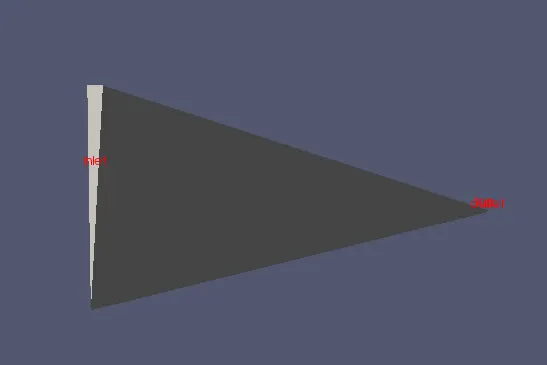
blockMesh command is used to create the mesh for the given geometry. Once the mesh is created successfully, execute the icoFoam command in the terminal with the case setup file open in the run folder of OpenFOAM.
Results and discussions:
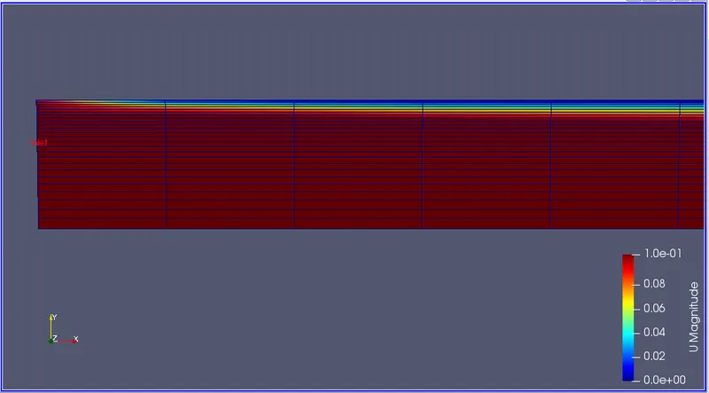
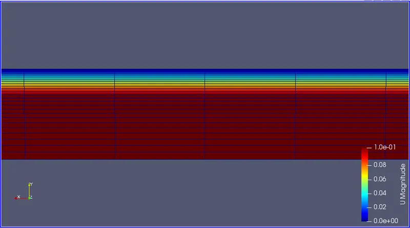
1. Velocity contours:
Entry region:
Fully developed region:
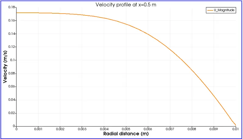
2. Velocity profiles:
Entry region:
Fully developed region:
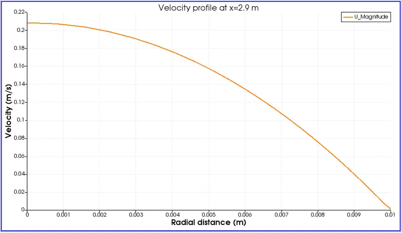
From these two plots, it is obvious that the velocity profile becomes more parabolic in the fully developed region. Near the wall (0.01m), the velocity is almost zero due to the friction between the fluid and the wall. As the radial distance from the center decreases, the velocity increases parabolically.
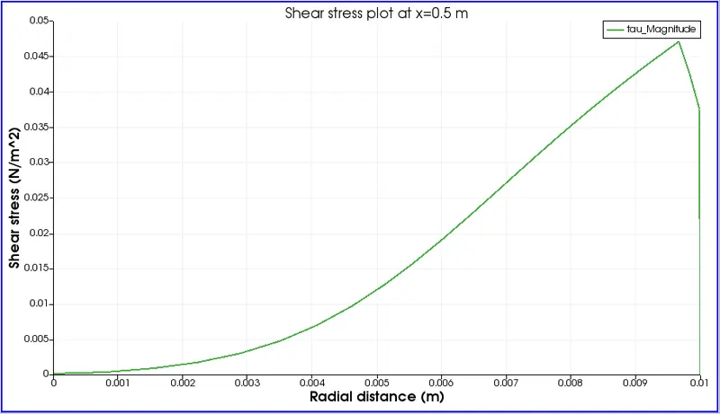
3. Shear stress plots:
Entry region:
Fully developed region:
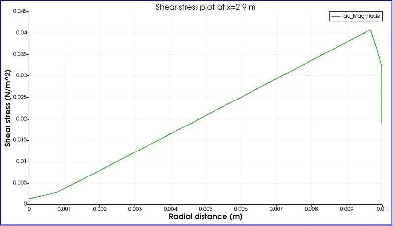
The shear stress is maximum at the wall and almost zero at the center. This is because there is more friction at the wall surface and the velocity gradient is more.
Validation:
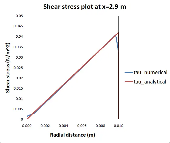
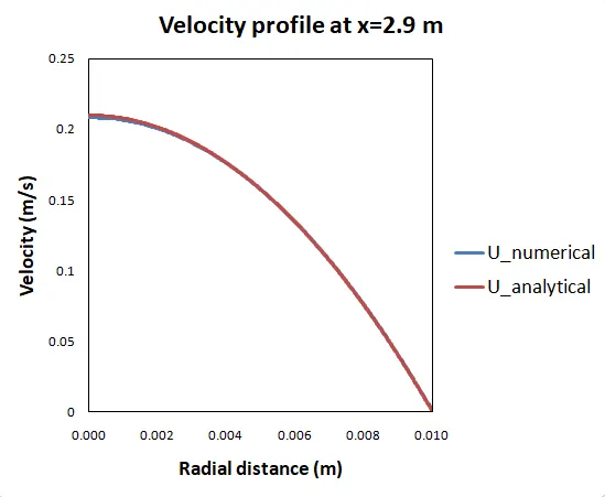
For a fully developed region, the numerical and analytical solutions are compared graphically.
Analytical solution:
- Average velocity `V_(avg) = (Re * mu)/(rho*D)` = 0.105 m/s
- Maximum velocity `V_(max) = 2 * V_(avg)` = 0.21 m/s
- Pressure drop `Deltap = (8*mu*L_(fdr)*V_(avg))/(r^2)` = 1.89 Pa
- Kinematic pressure drop `Deltap_k = (Deltap)/rho` = 0.006102 `m^2`/`s^2`
- Wall shear stress `tau = (f/4)*((rho*V_(avg)^2)/2)` = 0.04 Pa
The velocity at any radial distance is given by,
`V(r) = V_(max)[1-(r/R)^2]`m/s
The shear stress is given by,
`tau=mu*((dV)/(dr))` `N/m^2`
The maximum values of velocity and shear stress are as follows:
| Parameter | Numerical value | Analytical value | % Difference |
| Velocity (m/s) | 0.208205 | 0.21 | 0.85 |
| Shear stress (`N/m^2`) | 0.0322027 | 0.042 | 0.23 |
Velocity profile (fully developed region):
Shear stress plot (fully developed region):