Week 3 - External flow simulation over an Ahmed body.
EXTERNAL FLOW SIMULATION OVER AN AHMED BODY
AIM:
To simulate the flow over an Ahmed body by using a steady-state solver and also to perform a grid independency test.
IMPORTANCE OF AHMED BODY:
The flow around road vehicles under normal operating conditions is principally turbulent which is characterized by large-scale operation and recirculation regions, complex wake flows, long trailing vortices, and interaction of boundary layer flow on vehicle and ground. In aerodynamic flow around a vehicle, it is a three-dimensional flow and the design will have an influence on principle features such as the shape of the vehicle, aerodynamic drag, fuel consumption, noise production, and road handling. By using wind tunnel experiments the designer have an understanding of airflow around the vehicle through extensive testing. But wind tunnel testing for every prototype is a time-consuming and costly process. In order to reduce time, it is necessary to use a simplified computational technique and adopt a model to describe the mean effect of turbulence. Unfortunately, a simple turbulence model often fails to calculate the flow properly especially the position of flow separation. To overcome the problem. S. R. Ahmed in 1984 described an Ahmed body with the standard results to test the various types of challenges and turbulence models.
The Ahmed body is a bluff body whose shape is simple enough to model while maintaining certain important car-like geometry features. Ahmed body is widely used in vehicle aerodynamics to validate the numerical model with the experimental data from wind tunnel testing available for the same. Once the numerical model is validated it is used to design new models of the ground vehicles.
CALCULATION OF Y+:
1. Skin friction coefficient `C_f` = 0.0576 `Re^(-1/5)`
2. Wall shear stress `tau_w` = `1/2.C_f.rho.(U_infty)^2`
3. `U_T` = `sqrt(tau_w/rho)`
4. Y+ = `(y . U_T)/nu` `->` y = `(Y+ . nu)/U_T`
Reynolds number - for default material (air)
Re = `(rho. u.D)/mu` = `(u.D)/nu` = `(1.225 * 1.044.25)/(1.7894e^(-5))` = 1786772.102 (Turbulent in nature)
`C_f` = `3.236e^(-3)`
`tau_w` = 1.23878
`U_T` = 1.0056
For the k-omega SST turbulence model, Y+ is assumed as 1.
The first layer thickness over the Ahmed body is calculated as follows:
y = `(Y+ * nu)/U_T` = `(1*1.7684e^(-5))/(1.225*1.0056)` = `1.426e^(-5)`
SOLVING AND MODELING APPROACH:
The analysis of external flow over Ahmed body is carried out in steady-state. Initially. basic mesh is used in the discretization of the domain to generate baseline simulation. Then step by step the mesh quality is improved until the results remain the same. The pressure contour, velocity contour, and coefficient of drag plot are generated. K-Omega turbulence model is chosen for the current analysis. This model takes elliptic near-wall behaviour meaning that it has an inherent nature of being able to communicate with the wall and actually has Dirichlet boundary condition.
GEOMETRY:
The pre-processing starts with importing the geometry of Ahmed body into Spaceclaim. After importing the geometry, it is very well known that we are simulating external flow simulation hence it requires an outer fluid domain. This can be done by using an enclosure. After creating the enclosure, it is required to remove the body on which external flow simulation has to be carried out if we are not interested in the flow inside the body. The inlet will be from 2m ahead of the body and the outlet will be 5m from the body. The side distances from the body are 0.5m and bottom is zero. After completing the first enclosure it is important to have another enclosure to have better mesh resolution near the body.
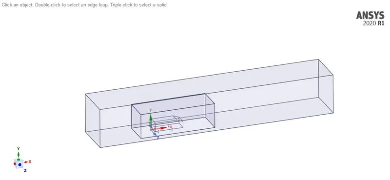
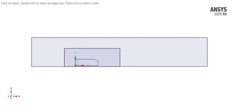
Overlapping of enclosures with each other is not acceptable for simulation. This can be overcome by using the interference option in Spaceclaim.
MESHING:
After completing geometry cleanup for simulation, the meshing is done. Multizone is selected.
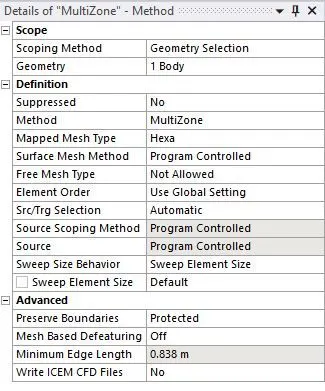
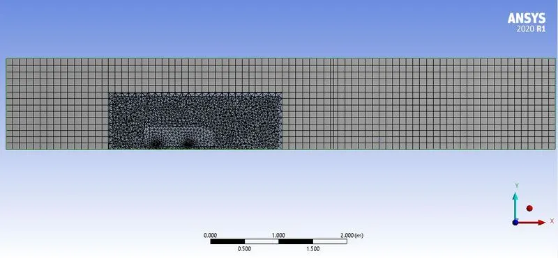
For the outer enclosure, the mesh element size is chosen as 0.1m. For the inner enclosure, the element size is chosen as 5e-2m (Tetragonal). The Ahmed body legs are further refined to an element size of 5e-3m. The total number of inflation layers is chosen as 6 with a first layer thickness value of 1.426e-5 as calculated before. For better resolution, the total layer thickness is chosen and its value is 3.5483e-5m. The growth rate is 1.2.
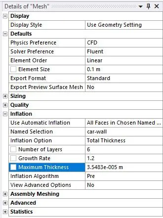
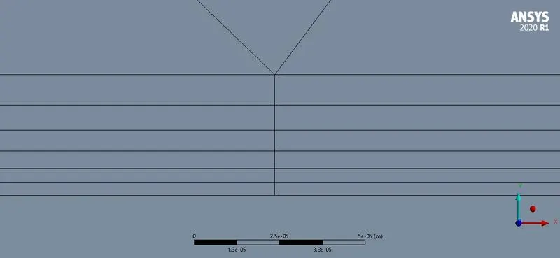
Totally four cases are studied in the current project. Initially, the mesh count is 0.2 million (203019 cells) with 51696 nodes.
| CASE 1 | CASE 2 | CASE 3 | CASE 4 | |
| OUTER ENCLOSURE | 0.1 m (Multizone) | 0.1 m (Multizone) | 0.1 m (Multizone) | 0.1 m (Multizone) |
| INNER ENCLOSURE | 5e-2 m (Tet) | 4e-2 m (Tet) | 3.5e-2 m (Tet) | 3.5e-2 m (Tet) |
| AHMED BODY PILLARS | 5e-3 m | 5e-3 m | 4e-3 m | 2e-3 m |
| FIRST LAYER THICKNESS | 1.426e-5 m | 1.426e-5 m | 1.426e-5 m | 1.426e-5 m |
| TOTAL THICKNESS | 3.5483e-5 m | 3.548e-5 m | 6.1315e-5 m | 6.1315e-5 m |
| GROWTH RATE | 1.2 | 1.2 | 1.2 | 1.2 |
| NO. OF LAYERS | 6 | 6 | 9 | 9 |
| TOTAL NODES | 51696 | 79811 | 117575 | 188409 |
| TOTAL ELEMENTS | 203019 | 303832 | 455187 | 678764 |
SOLVER SETUP:
For the solver setup, a pressure-based solver is used rather than a density-based solver by calculating the Reynolds number. The fluid which is used throughout the simulation is Air. The inlet boundary condition is considered as velocity inlet of 25 m/s and the outlet boundary condition is considered as pressure outlet (atmospheric pressure). It is necessary to define the car wall as a boundary of the wall with no-slip conditions to evaluate the drag coefficient. For reference values, the frontal area of the Ahmed body 0.131482 `m^2` is provided as area and the length is given as 1.044 m. The SIMPLE algorithm is chosen for the pressure-velocity coupling. For solution animation, a reference frame or plane is required on which the results are displayed. This can be done by using the location option in which a plane is created for reference.
POST-PROCESSING:
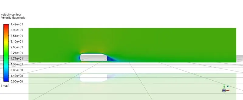
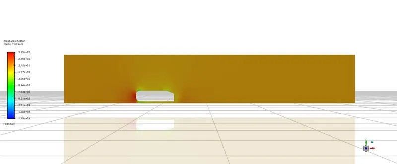
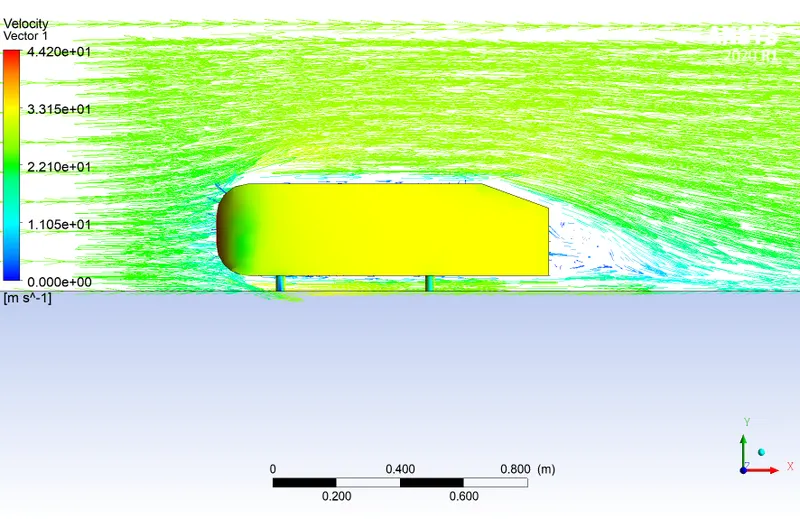
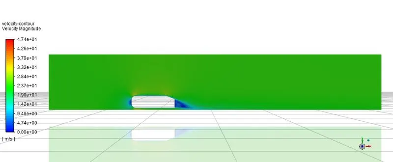
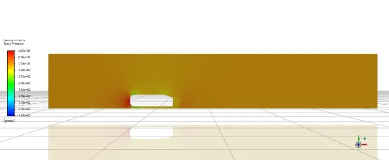
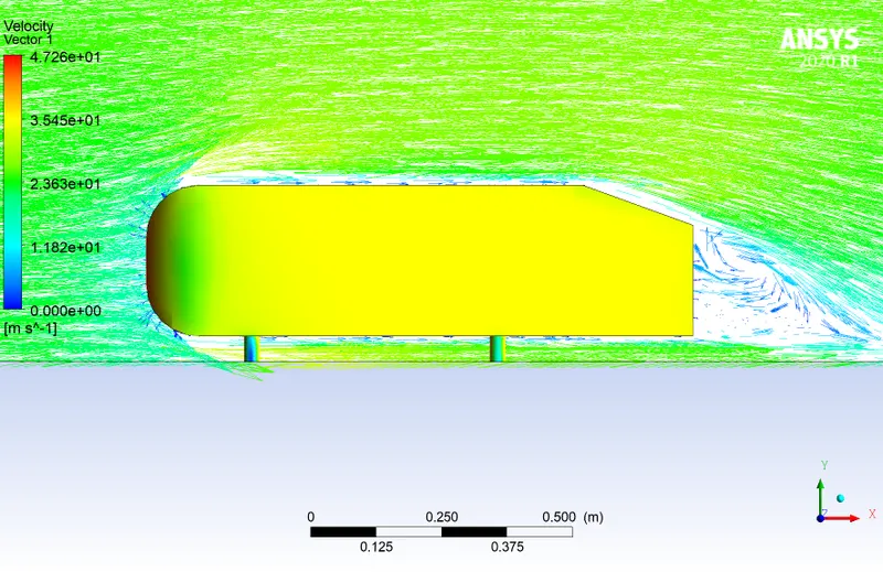
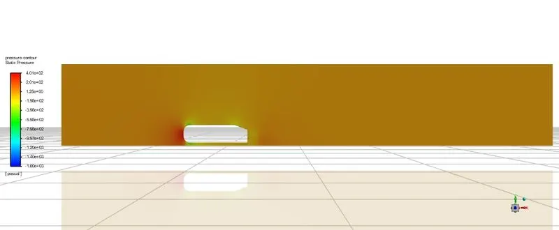
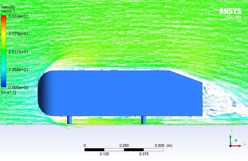
In post-processing, all velocity, and pressure contours with vector plots are used to study the flow in the wake region and point of separation from the Ahmed body model.
CASE 1:
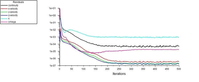
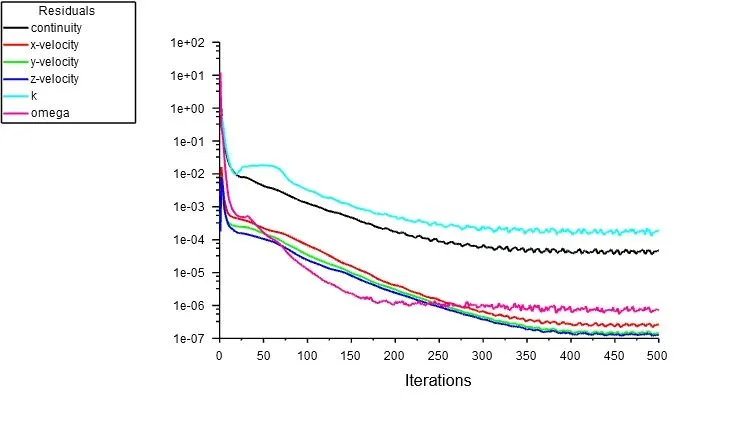
1. Residuals
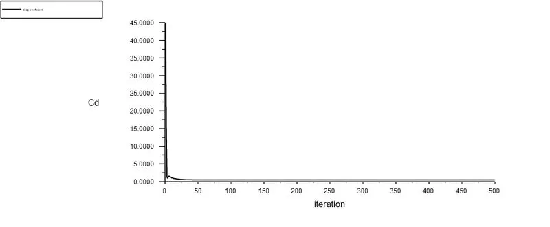
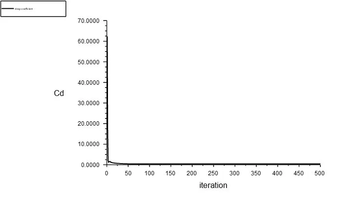
2. Drag coefficient
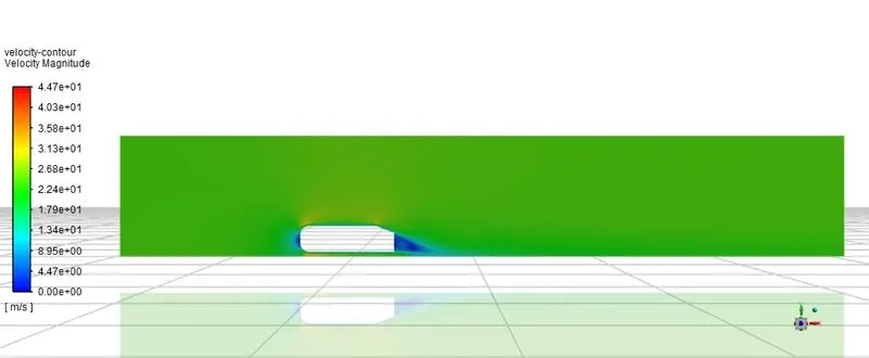
3. Velocity contour
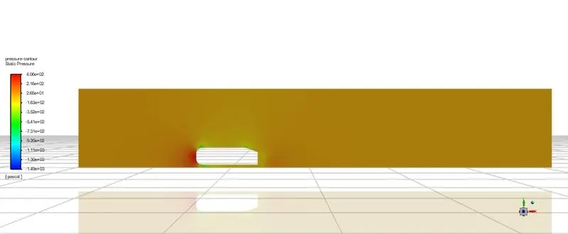
4. Pressure contour
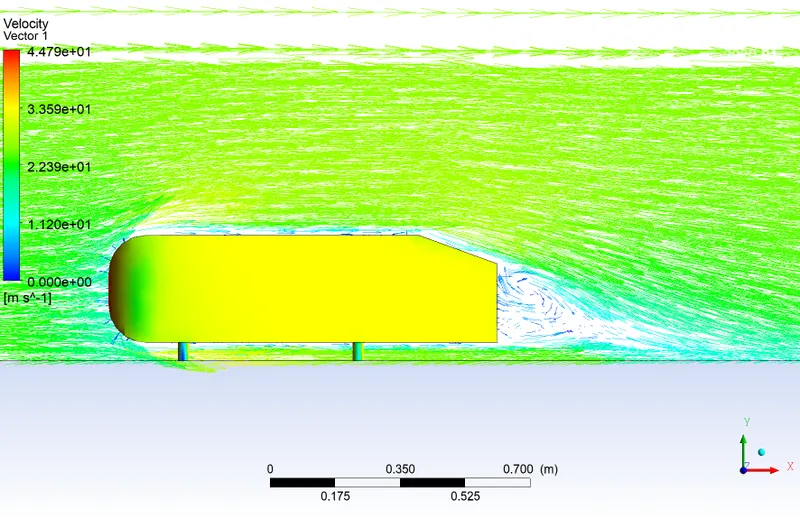
5. Vector plot
CASE 2:
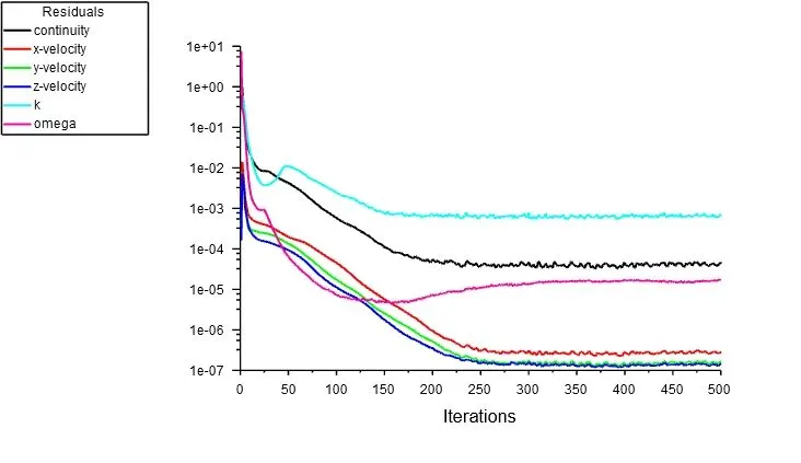
1. Residuals
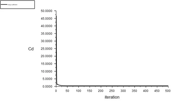
2. Drag coefficient
3. Velocity contour
4. Pressure contour
5. Vector plot
CASE 3:
1. Residuals
2. Drag coefficient
3. Velocity contour
4. Pressure contour
5. Vector plot
CASE 4:
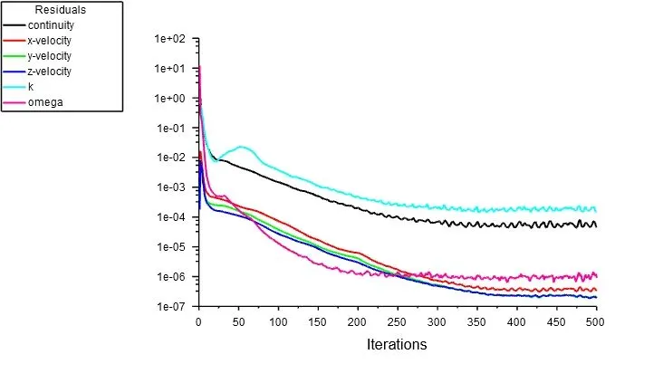
1. Residuals
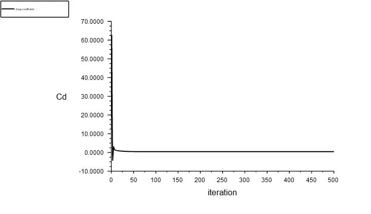
2. Drag coefficient
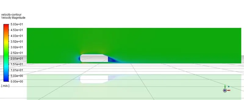
3. Velocity contour
4. Pressure contour
5. Vector plot
VELOCITY ANIMATION:
GRID INDEPENDENCE TEST:
| CASE | ELEMENTS | DRAG COEFFICIENT |
| 1 | 203019 | 0.48 |
| 2 | 303832 | 0.45 |
| 3 | 455187 | 0.42 |
| 4 | 678764 | 0.42 |
As the number of elements increases the drag coefficient value decreases and remains constant with very minimum deviation. Thus the current study is independent of the grid. Cases 3 and 4 provide more accurate results when compared to other cases because of the better mesh resolution.
NEGATIVE PRESSURE IN THE WAKE REGION:
A high-pressure region is observed in the front portion of the Ahmed body and a drop in pressure is observed when the flow leaves the Ahmed body at the rear portion. This can be illustrated using the flow over an airfoil structure.
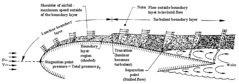
The detachment of flow at the rear end results in the formation of eddies. The region behind the Ahmed body where the flow is unstable is called the wake region, where the pressure adversely drops.
At the inlet, fluid flows with a velocity of 25 m/s. When it encounters the Ahmed body in the front, the flow gets stagnated and there is a reduction in velocity leading to an increase in pressure. The fluid that comes into contact with the body behaves like a viscous sublayer and this property of the fluid remains until it is in contact with the body. At the slant of the Ahmed body, the fluid separates the body and the point of separation is created.
When the fluid flows over the body, the boundary layer thickness increases. The fluid layer adjacent to the wall causes surface friction by consuming some kinetic energy. This loss of kinetic energy can be recovered from the adjacent fluid layer through the momentum exchange process. Thus the velocity of the layer goes on decreasing. Along the length of the body, at a certain point, a stage may come when the boundary layer gets separated from the surface. This phenomenon is called boundary layer separation.
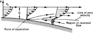
Near the surface of the solid when the point of separation occurs the fluid is incapable of sticking on the surface. This leads to the point where pressure reduces to negative. This induces extra drag force at the rear which creates a loss in the velocity of the fluid and reduces the velocity of the body. This negative pressure in the rear gives rise to vortices and eddies which creates losses. For this reason, in most cases, the point of separation of the boundary layer is designed in such a manner to create the negative pressure away from the boundary.
Conditions for boundary layer separation:
| PRESSURE GRADIENT | VELOCITY GRADIENT | |
| NO BOUNDARY LAYER SEPARATION | `(partialp)/(partialx)<0` | `(partialu)/(partialy)>0` |
| ON THE VERGE OF SEPARATION (POINT OF SEPARATION) | `(partialp)/(partialx)=0` | `(partialu)/(partialy)=0` |
| BOUNDARY LAYER SEPARATION | `(partialp)/(partialx)<0` | `(partialu)/(partialy)<0` |
SIGNIFICANCE OF POINT OF SEPARATION:
The point on the body where the boundary layer lifts off the surface is called the separation point. When the airflow separates off the surface, the pressure drag usually increases. The separation point is the point where the air stops sticking to an object that is moving through the air. When an object is moving through the air, the air molecules push back on it and resist the object's movement - this resistance is called pressure drag.
The position of the point of separation plays an essential role in the case where one wants less aerodynamic drag. To achieve this we can find several examples that are implemented in recent years like the continuous shape of an outer layer of the body, providing wings, flaps, slats to locate the point of separation away from the body. The arrangements changes from application to application but the basic idea behind it is to reduce the drag as much as possible and make the object aerodynamically stable. After the point of separation, the formation of eddies starts.
CONCLUSION:
- The grid independence test is carried out to demonstrate the variation of the result with respect to the accuracy of the mesh. Good quality mesh is needed for achieving accurate results.
- The inflation layer provided is an added advantage to capture the flow near the Ahmed body.
- The cause of flow separation in the fluid flow is because of the negative pressure generated in the boundary layer of flow near the wall of the body and the negative wake region is generated due to the pressure difference between a low stream and high stream flow also due to flow separations.