Week 5 - Rayleigh Taylor Instability

RAYLEIGH-TAYLOR INSTABILITY

Introduction:

The Rayleigh-Taylor instability is the instability of an interface between two fluids of different densities which occurs when the lighter fluid is pushing the heavier fluid. As the RT instability develops, the initial perturbations progress from a linear growth phase into a non-linear growth phase, eventually developing 'plumes' flowing upwards (in the gravitational buoyancy sense) and 'spikes' falling downwards. In the linear phase, the fluid movement can be closely approximated linearly, and the amplitude of perturbations is growing exponentially with time. In the non-linear phase, perturbation amplitude is too large for a linear approximation, and nonlinearity is required to describe fluid motions.

Water suspended atop oil is an everyday example of Rayleigh-Taylor instability, and it may be modeled by two completely plane-parallel layers of immiscible fluid, the denser fluid on top of the less dense one and both subject to the Earth's gravity. The equilibrium is unstable to any disturbances of the interface. If a parcel of heavier fluid is displaced downward with an equal volume of lighter fluid displaced upwards, the potential energy of the configuration is lower than the initial state. Thus the disturbance will grow and lead to a further release of potential energy, as the denser material moves down under the effect of the gravitational field, and the less dense material is displaced upwards. The following image shows a typical RT instability case.

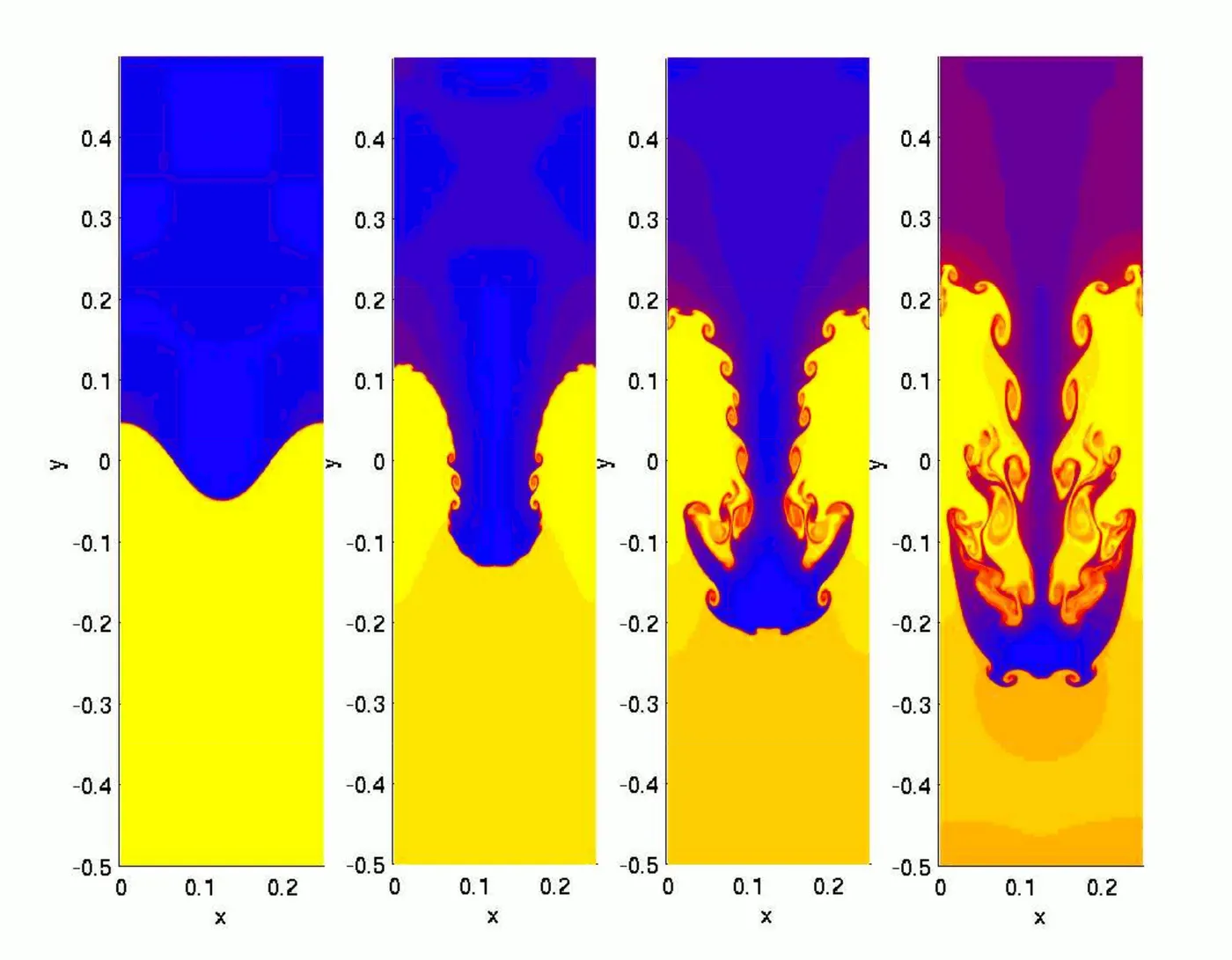
Different examples of RT instability in real life are as follows: A mushroom cloud in volcanic eruptions, atmospheric nuclear explosion, supernova explosion in outer space, instabilities in plasma fusion, and inertial confinement fusion.

CFD models based on mathematical analysis of RT instability:

1) Volume of Fluid (VOF)

In CFD, the Volume of Fluid (VOF) method is a free surface modeling technique for tracking and locating the free surface or fluid-fluid surface. It belongs to the class of Eulerian methods which are characterized by a mesh that is either stationary or is moving in a certain prescribed manner to accommodate the evolving shape of the interface.

2) K-L Turbulence model

The K-L model was proposed by Dimonte and Tipton for describing the turbulent self-similar regime of RT and RM-induced mixing. The model describes the dominant eddies in the mixing zone with evolutionary equations for their characteristic dimension (L) and energy per unit mass (K).

3) Kelvin-Helmholtz/Rayleigh Taylor Hybrid model

This model was used to predict the primary break up of the intact liquid core of the jet and the Rayleigh Taylor model determines the effects of acceleration of the different phases. This model predicts the shape of the spray considering the temperature at different places.

Procedure:

The following procedure is followed in setting up a simulation

Geometry

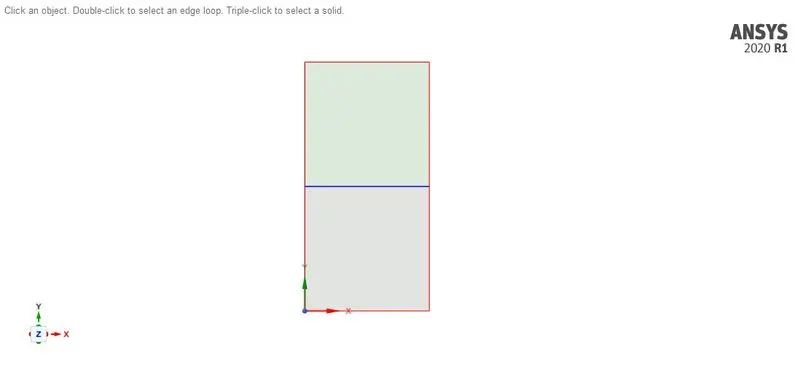
Two components are created using the surface pull option each of 20mm x 20mm sharing a common edge.

Mesh

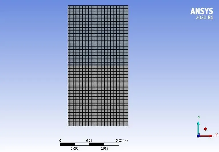
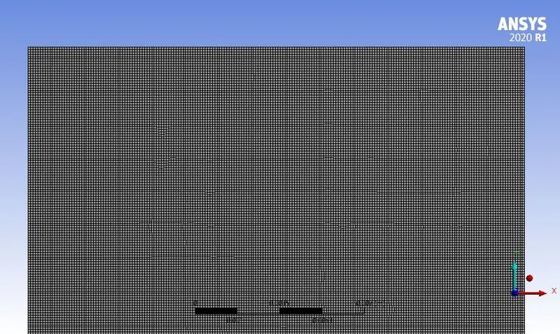
A basic quad mesh is created. Mesh size for each case is as follows:

Case A - 0.5mm

Case B - 0.1mm

Case C - 0.1mm

Mesh size	Nodes	Elements
0.5mm	3486	3362
0.1mm	80601	80000

Setting up physics

Transient, Pressure-based solver. Multiphase is activated. The implicit method is chosen. The primary phase is air and the secondary phase is water.

Initialization

Standard initialization is used. Then the water is patched to the air and water surfaces as VOF 0 and 1 respectively.

Results:

Effect of mesh size

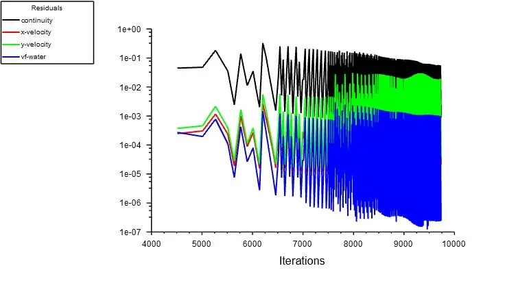
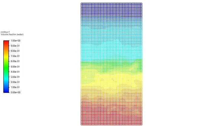
1) CASE A: Mesh size = 0.5mm; Air + Water

Residuals plot:

Phases contour:

Animation:

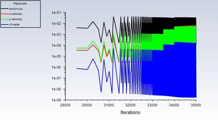
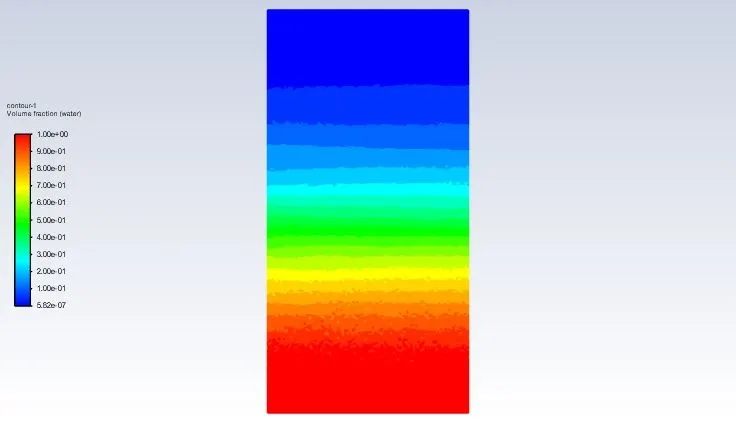
2) CASE B: Mesh size = 0.1mm; Air + Water

Residuals plot:

Phases contour:

Animation:

Effect of density

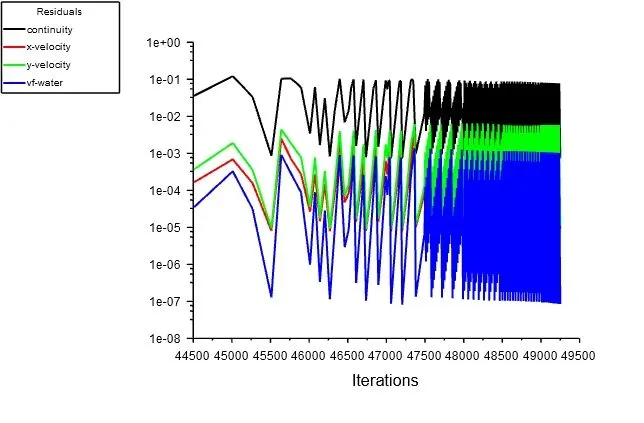
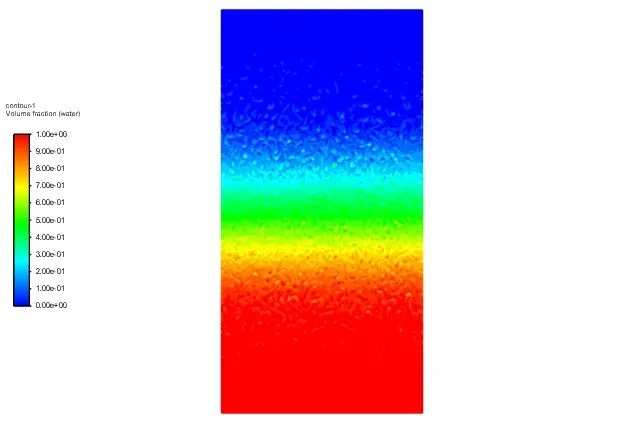
3) CASE C: Mesh size = 0.1mm; User-material + Water

Residuals plot:

Phases contour:

Animation:

Why steady-state simulation is not suitable?

• We know that a steady-state simulation is a time-independent approach
• Based on the simulation, we know that there is high turbulence, and the flow change occurs between very small time variations. It is impossible to capture in steady-state simulation.
• Also, the steady-state solver ignores the time differential terms involved in the simulation. Therefore, even if it can capture the state of equilibrium, it doesn't capture the non-linearities in the simulation precisely.

Atwood number:

It is a dimensionless number in fluid dynamics that are used to study hydrodynamic instabilities in density stratified flows.

`A=(rho_1-rho_2)/(rho_1+rho_2)`

Case B (Air + Water):

`rho_1` = 998

`rho_2` = 1.225

A = 0.99754

Case C (User-material + Water):

`rho_1` = 998

`rho_2` = 400

A = 0.42775

Effect of Atwood number:

• When A is near 1, there is a clear formation of the bubble of low-density fluid and spikes of high-density fluid.
• When A is away from 1, it is difficult to differentiate between the bubbles and spike due to less density difference.
• Also, the simulation attains equilibrium quickly when A is close to 1 whereas the equilibrium time increases considerably when A is distant from 1 as the fluid mixes too well.