Week 9 - FVM Literature Review

FINITE VOLUME METHOD - LITERATURE REVIEW

The conservation laws of fluid motion are described either in differential form or in integral form. When the integral form of governing equations are solved, the domain is divided into small volumes. In these elementary volumes, the conservation laws can be applied. This is called the Finite Volume Method (FVM).

FDM VS FVM:

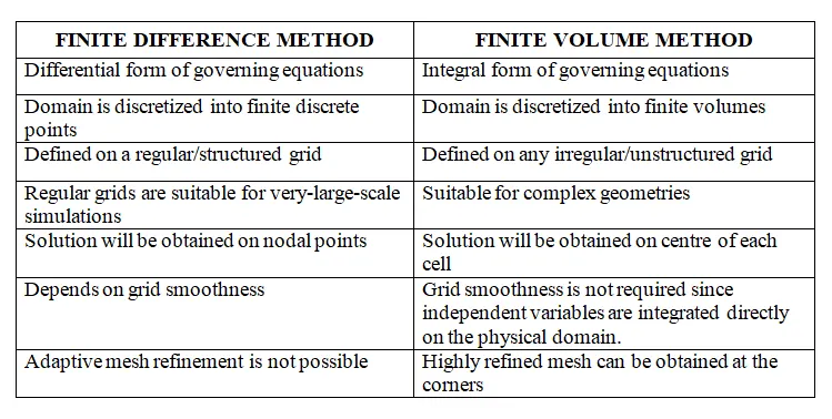
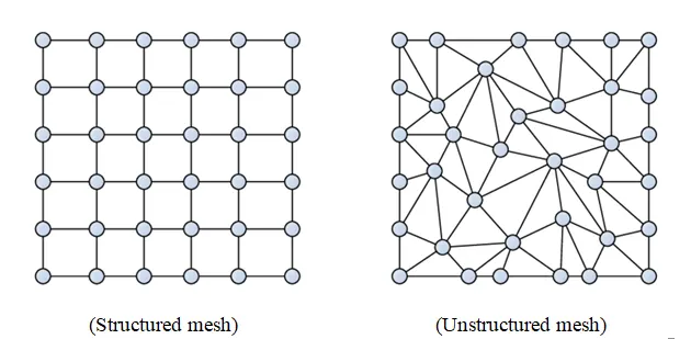
The finite volume method is explained with an example of a 1D steady-state diffusion problem (1D Heat conduction).

1D linear heat conduction problem:

Neglecting the unsteady term and convective term,

div (`Gamma`grad`phi`) + `S_phi` = 0

Applying control volume integration yields the following equation:

`int_(C.V)` div (`Gamma`grad`phi`) dV + `int_(C.V)``S_phi` dV = 0

Using Gauss-divergence theorem,

`int_A` n(`Gamma`grad`phi`) dA + `int_(C.V)``S_phi` dV = 0

Consider steady state diffusion of property `phi` in a 1D domain.

The governing equation is,

`d/dx[Gamma(dphi)/dx] + S = 0`

where, `Gamma` `->` diffusion coefficient; S `->` source term

Boundary values A and B are prescribed.

For 1D heat conduction problem, replace `Gamma -> k` (thermal conductivity); `phi -> T` (Temperature); `S -> q` (heat generated)

Step1: Grid generation

The first step in the finite volume method is to divide the domain into discrete control volumes. Let us place a number of nodal points in the space between A and B. The boundaries (or faces) of control volumes are positioned mid-way between adjacent nodes. Thus each node is surrounded by a control volume or cell. It is common practice to set up control volumes near
the edge of the domain in such a way that the physical boundaries coincide with the control volume boundaries.

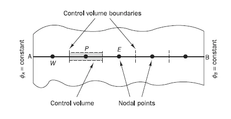
P `->` present node

E `->` east node

W `->` west node

P, W, E `->` nodal points

p, w, e `->` faces

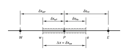
The distances between the nodes W and P, and between nodes P and E, are identified by `deltax_(WP)` and `deltax_(PE)` respectively. Similarly, distances between face w and point P and between P and face e are denoted by `deltax_(wP)` and `deltax_(Pe)` respectively. The control volume width is Δx = `deltax_(we)`.

Step2: Discretisation

`int_(DeltaV)``d/dx(Gamma(dphi)/dx) dV` + `int_(DeltaV)` S dV = 0

`=>` `int_w^e``d/dx(Gamma(dphi)/dx) A dx` + `int_(DeltaV)` S dV = 0

`=>` `[(Gamma A (dphi)/dx)_e - (Gamma A (dphi)/dx)_w] + overlineS DeltaV = 0`

`Gamma_e A_e ((dphi)/dx)_e - Gamma_w A_w ((dphi)/dx)_w + overlineS DeltaV = 0`

For 1D heat conduction,

`k_e A_e ((dT)/dx)_e - k_w A_w ((dT)/dx)_w + overlineq DeltaV = 0`

The values of k and T are defined and evaluated at the nodal points. These values require information from the neighbouring ponits.

To solve the T from `(dT)/dx` `->` gradient scheme is used since it directly depends on the values of T from neighbouring points.

For the diffusion coefficient which is a function of the property (T) which inturn requires information from the neighbouring points, the interpolation scheme is used.

For 1D steady state diffusion, it is sufficient to use forward differencing for the property `phi` and central differencing for the diffusion coefficient `Gamma`.

`therefore` `Gamma_w = (Gamma_W+Gamma_P)/2` and `Gamma_w = (Gamma_W+Gamma_P)/2`

`((dphi)/dx)_e=(phi_E-phi_P)/(deltax)_(PE)`

`((dphi)/dx)_w=(phi_P-phi_W)/(deltax)_(PW)`

Note: The above schemes will not work all the times. `therefore` we go for certain interpolations schemes which will be discussed later.

In practical situations,the source term S may be a function of the dependent variable. In such cases the finite volume method approximates the source term by means of a linear form:

`overlineSDeltaV = S_u + S_P phi_P`

`Gamma_eA_e[(phi_E-phi_P)/(deltax)_(PE)] - Gamma_wA_w[(phi_P-phi_W)/(deltax)_(PW)] + overlineS DeltaV = 0`

`Gamma_eA_e(phi_E)/(deltax_(PE)) - Gamma_eA_e(phi_P)/(deltax_(PE)) - Gamma_wA_w(phi_P)/(deltax_(PW)) + Gamma_wA_w(phi_W)/(deltax_(PW)) + S_u + S_Pphi_P = 0`

`(Gamma_eA_e)/(deltax_(PE))phi_P + (Gamma_wA_w)/(deltax_(PW))phi_P - S_Pphi_P = (Gamma_wA_w)/(deltax_(PW))phi_W + (Gamma_eA_e)/(deltax_(PE))phi_E+ S_u`

Identifying the coefficients of `phi_W` and `phi_E` as `a_W` and `a_E`, and the coefficient of `phi_P` as `a_P`, the above equation can be written as

`(a_W + a_E - S_P)phi_P = a_Wphi_W + a_Ephi_E + S_u`

`a_Pphi_P = a_Wphi_W + a_Ephi_E + S_u`

where,

`a_W`	`a_E`	`a_P`
`(Gamma_wAw)/(deltax)_(WP)`	`(Gamma_eAe)/(deltax)_(PE)`	`a_W + a_E - S_P`

Step3: Solution of equations

The resulting system of linear algebraic equations is then solved to obtain the distribution of the property `phi` at nodal points. Any suitable matrix solution technique may be enlisted for this task.

INTERPOLATION SCHEMES:

The approximations of surface and volume integrals require values of the variable at a location other than the computational nodes of the control volume. Values at these nodes are obtained using interpolation formulae. Some of the interpolation methods are as follows:

• Upwind interpolation
• Linear interpolation
• Quadratic Upwind Interpolation for Convection Kinematics
• Hybrid, TVD, and ENO interpolation schemes

1. Upwind interpolation (UDS)

In this scheme, values from the upwind/upstream of the cell centers should be defined. It is used in convection dominated problems. The upwind interpolation for approximating the value of a variable f at the east face of a control volume is given by

`f_e ={(f_P,if,(v, n)_e,>,0),(f_E,if,(v,n)_e,<,0):}`

This interpolation scheme is equivalent to the forward differencing method or backward differencing method depending on the flow direction.

If the flow is along the -ve x-direction, then the values at the interface are given by

for v<0;

`u_(i+1/2) ~~ u_i` ; `u_(i-1/2) ~~ u_(i-1)`

`I_c = v (u_i - u_(i-1))/(Deltax)` which is equivalent to Backward differencing scheme

If the flow is along the +ve x-direction, then the values at the interface are given by

for v>0;

`u_(i-1/2) ~~ u_(i-1)` ; `u_(i+1/2) ~~ u_i`

`I_c = v (u_(i-1) - u_i)/(Deltax)` which is equivalent to Forward differencing scheme

It is said to be equivalent because all three methods have an order of accuracy 1.

Advantage:

• UDS is the only approximation that satisfies the boundedness criterion unconditionally irrespective of velocity and grid spacing i.e. never yield oscillatory solutions.

Disadvantages:

• UDS is numerically diffusive
• Numerical diffusion is magnified in multi-dimensional problems if the flow is oblique to the grid
• Peaks or rapid variations in the variables will be smeared out
• Only first-order accurate, hence very fine grids are required to obtain accurate solutions.

2. Linear interpolation (CDS)

In this scheme, approximate values of the variable at the face center of the control volume are obtained by the linear interpolation of the values from the two nearest computational nodes (one upstream and one downstream).

`f_e = f_Elambda_e + f_P(1-lambda_e)`

where, `lambda_e = (x_e - x_p)/(x_E - x_P)`

It is more simple and widely used.

The linear interpolation is equivalent to the use of the central differencing formula of the first-order derivative and hence this scheme is also termed as Central Differencing Scheme (CDS)

Average interface values are given by

`u_(i+1/2) = (u_i + u_(i+1))/2`

`u_(i-1/2) = (u_(i-1) + u_i)/2`

`I_c = v (u_(i+1) - u_(i-1))/(2Deltax)` which is equivalent to CDS.

It is said to be equivalent because both these methods have an order of accuracy 2.

Advantages:

• Approximation of gradients has second-order of accuracy on uniform grids
• It's formally of first-order on non-uniform grids

Disadvantage:

• It may produce oscillatory solutions in case of large grid space

3. Hybrid interpolation scheme

It is a blend of UDS and CDS. The hybrid differencing scheme exploits the favorable properties of the upwind and central differencing schemes. It switches to upwind differencing when central differencing produces inaccurate results at high Pe numbers.

The scheme is fully conservative and since the coefficients are always positive it is unconditionally bounded. It satisfies the transportiveness requirement by using an upwind formulation for large values of Peclet number.

`f_e = gamma f_(CDS) + (1-gamma)f_(UDS)`

Advantage:

• Produces physically realistic solutions and highly stable compared to QUICK

Disadvantage:

• Accuracy is of first-order

4. Quadratic Upwind Interpolation for Convective Kinematics (QUICK)

It approximates the values of the variable at the face center of a CV by quadratic interpolation of the values at three nearest computational nodes (1 downstream node D & 2 upstream nodes U, UU)

Quadratic - As it uses 3 nodes

Upwind - As it uses two upstreams

Convective Kinematics - As it is used for convective domain problems

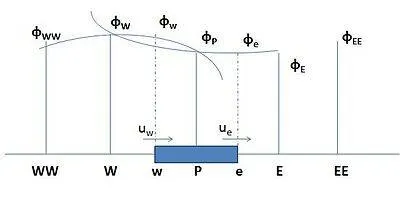
for `u_w > 0`

`phi_w` is evaluated based on the values at WW, W, and P

for `u_e > 0`

`phi_e` is evaluated based on the values at W, P, and E

for `u_w < 0`

`phi_w` is evaluated based on the values at W, P, and E

for `u_e < 0`

`phi_e` is evaluated based on the values at P, E, and EE

`f_e = f_E + g_1 (f_D - f_U) + g_2(f_(UU) - f_U)`

where,

`g_1=((x_e-x_U)(x_e-x_(UU)))/((x_(UU) - x_U)(x_(UU) - x_D))`

`g_2=((x_e-x_U)(x_e-x_(D)))/((x_(UU) - x_U)(x_(UU) - x_D))`

Advantages:

• It is the better version of UDS and CDS because it is more accurate than UDS and more damping in nature than CDS as it uses 3 nodes to solve
• It has an order of accuracy 3

Disadvantages:

• The use of QUICK can lead to subtle problems caused by unbounded results
• Implementation of boundary conditions could be problematic with such higher-order schemes

5. Total Variation Diminishing scheme (TVD)

The fact that the QUICK scheme and other higher-order schemes can give overshoots and undershoots has led to the development of second-order schemes that avoid these problems. The class of Total Variation Diminishing (TVD) scheme has been specifically formulated to achieve oscillation-free solutions and has proved to be useful in CFD calculations.

TVD scheme is designed to address the undesirable oscillatory behavior of higher-order schemes. In the TVD scheme, the tendency towards oscillation is counteracted by adding an artificial diffusion fragment or by adding a weighting parameter towards upstream contribution. TCD has an order of accuracy 2.

`f_e = f_P + 1/2psi(r)(f_E - f_P)`

where,

`psi(r)` is called as flux limiter function

where,

`r = (u_i - u_(i-1))/(u_(i+1) - u_i)`

FLUX LIMITER:

For convective fluid flow, it is observed that the lower-order schemes are usually stable but quite dissipative in nature around the points of discontinuity or shocks while the higher-order schemes are unstable in nature and show oscillations in the vicinity of discontinuities or shocks. Highly accurate and oscillation-free schemes are knowns as high resolution schemes.

In order to make the scheme TVD, we must constrain or limit the range of possible values of the additional convective flux `f_e = f_P + 1/2psi(r)(f_E - f_P)`, which was originally introduced to make the scheme higher-order. Hence, the function `psi(r)` is called a flux limiter function.

Flux limiter functions are used to fine tune the higher order and lower order schemes in such a way that the resulting scheme gives a higher order accuracy in the smooth region of the flow and maintains first order accuracy in the vicinity of shocks and discontinuities.

`F(u_(i+1/2)) = f^(low)(i+1/2) - psi(r_i)(f^(low)(i+1/2) - f^(high)(i+1/2))`

`F(u_(i-1/2)) = f^(low)(i-1/2) - psi(r_i-1)(f^(low)(i-1/2) - f^(high)(i-1/2))`

where,

`f^(low)` is low precision flux (first order)

`f^(high)` is high precision flux (higher order)

CONCLUSION:

Finite Volume Method (FVM) is really a powerful approach to solve the CFD problems. With the help of a proper interpolation scheme and the accurate use of flux limiters in case of any discontinuities present, we can solve a wide range of CFD problems. Though it may be difficult to code and implement it in the computer, it gives an added advantage through its robustness.