Week 2 - Flow over a Cylinder.
SIMULATION OF FLOW OVER A CYLINDER
AIM:
- To simulate the flow with the steady-state and unsteady-state flow and calculate the Strouhal number for Re = 100. (PART I)
- To calculate the coefficient of drag `C_d` and coefficient of lift `C_l` by setting Re = 10, 100, 1000, 10000, and 100000 (with steady-state solver) and discuss the effect of Re on `C_d`. (PART II)
THEORY:
Karman vortex street:
The Karman vortex street is an exquisite flow pattern that can be seen in a variety of flow situations. Consider a stream of fluid flow past a circular cylinder, which can be called the archetypal or quintessential bluff body - a cross-section of 'perfect platonic circle'.
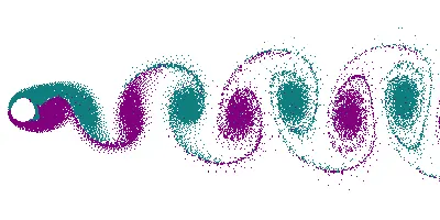
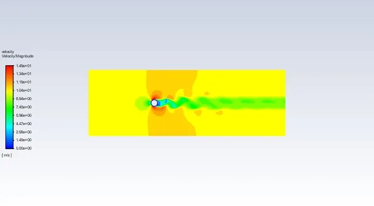
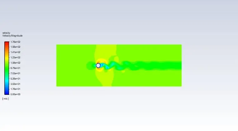
In the wake of the cylinder, the flow pattern consists of an alternating system of vortices or regions of rotation. A clockwise rotating eddy or vortex is shed from the top side, followed by an anti-clockwise rotating vortex from the bottom side, and this process continues leading to a staggered system of alternating vortices. It is important to notice that even if the oncoming flow is steady (i.e, does not change with time), the unsteadiness is intrinsically generated and the Karman street is formed downstream of the body.
The most dangerous aspect of the Karman vortex street is its periodic nature. It leads to possibilities of resonance with natural structural modes of flexible bodies and hence results in the failure of structures.
Strouhal number:
Strouhal, in 1878, made the first experiments of frequencies associated with the shedding of vortices. Strouhal measured the frequency of acoustic tones coming from a vertical wire that was made to revolve at uniform speed about a parallel axis, and showed that the origin of these acoustic tones is essentially aerodynamic. By varying the diameter (D) of the wire and the speed (V) of the wire motion, Strouhal found that (within certain limits) the acoustic frequency (f) was expressible as
`f = 0.185(V/D)`
In other words, the acoustic frequency is related directly to the periodic formation of vortices. The above relation also suggested that the non-dimensional number (fD/V) was approximately a constant (within the range of values) and has since become known as the Strouhal number.
`Sr = (fD)/V`
Physically,
Advection time/time characteristic of unsteadiness
When the fluid stream reaches roughly the topmost point of the cylinder, it finds itself unable to negotiate the rear half of the cylinder where there is an uphill pressure gradient. Hence the fluid separates from the top surface, constitutes itself into a clockwise swirling vortex as it approaches the rear end of the cylinder after which it peels off like a shed vortex. Hence the vortex forming time is proportional to the perimeter (or the diameter) of the cylinder.
PROCEDURE:
The present study involves two parts. In part-I, the flow over the cylinder is simulated with both steady and unsteady cases for Re = 100 and the Strouhal number `Sr` is calculated for both the cases. In part-II, the effect of Re on `C_d` is analyzed for a range of Re values (10, 100, 1000, 10000, & 100000) and to calculate the coefficient of drag and lift in each case. The workflow is as follows: Geometry `->` Meshing `->` Case setup `->` Solution `->` Results
Terminologies used:
Re `->` Reynold's number
`C_d` `->` Coefficient of drag
`C_l` `->` Coefficient of lift
V `->` Velocity of the fluid (m/s)
`V_(mp)` `->` Average velocity at the monitor point (m/s)
Sr `->` Strouhal number
Geometry:
A cylinder of 2m diameter is considered for the study. A 2D simulation is performed for ease in the calculation. The geometry is created in the SpaceClaim. Details of the geometry are shown in the following figure.
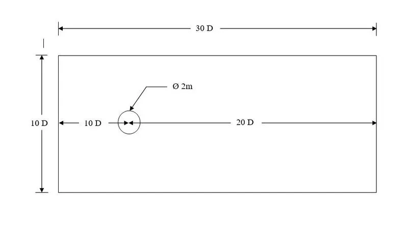
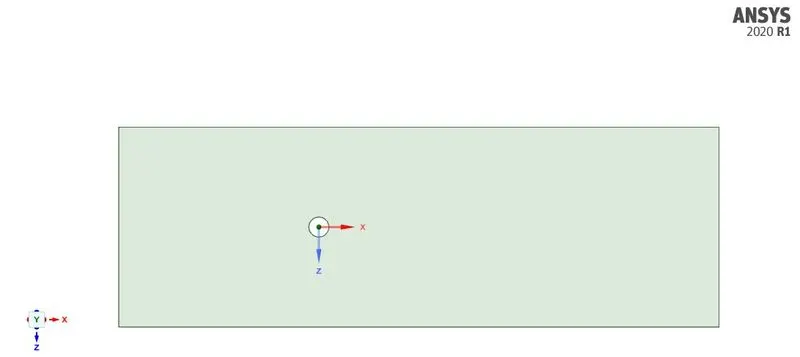
The geometry is created using the rectangle tool. Then the circle is created and the pull tool is used to convert it into a surface. The circle is cut out and the construction lines are deleted.
Meshing:
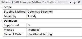
In the meshing window, the triangles method is selected and the element size is chosen as 0.25 m.
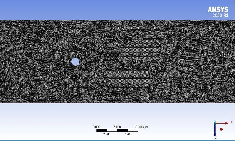
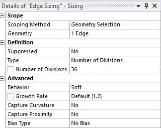
In the sizing method, the cylinder edge is selected and the number of divisions is given as 36.
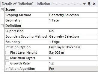
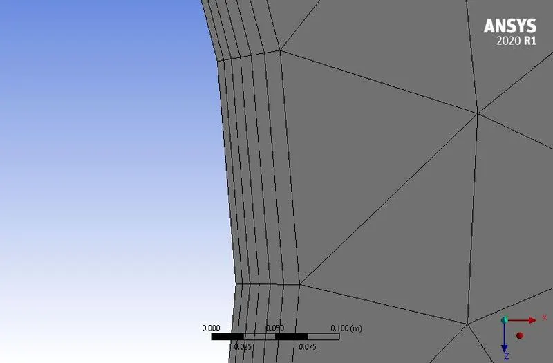
Then inflation layer is inserted. The first layer thickness is selected with a height of 5e-03 and a total of 6 layers. The growth rate is 1.2.
Case setup:
First, the type of simulation is selected whether steady or transient. A pressure-based solver with absolute velocity is chosen. The mesh check is run and the cell count is found to be 40502. In the viscous option, laminar is selected. In physics, new user material is defined as the study is performed for different values of Re by simply varying the velocity. The properties of the user-material are as follows:
Density `rho` = 1 kg/`m^3`
Dynamic viscosity `mu` = 0.02 `(N s)/m^2`
Reynold's number Re = `(rho V D)/mu`
The different cases involved in the present study are as follows:
Part-I:
| Case | Type | Re | V |
| 1a | Steady | 100 | 1 m/s |
| 1b | Unsteady | 100 | 1 m/s |
Part-II:
| Case | Type | Re | V |
| 2a | Steady | 10 | 0.1 m/s |
| 2b | Steady | 100 | 1 m/s |
| 2c | Steady | 1000 | 10 m/s |
| 2d | Steady | 10000 | 100 m/s |
| 2e | Steady | 100000 | 1000 m/s |
To study the vortex formation a monitor point is set at a distance of 8m from the center of the cylinder in the wake region. The following report definitions are created:
- Vertex average of monitor point velocity
- Coefficient of drag
- Coefficient of lift
Then the solution is initialized and the following contours are defined:
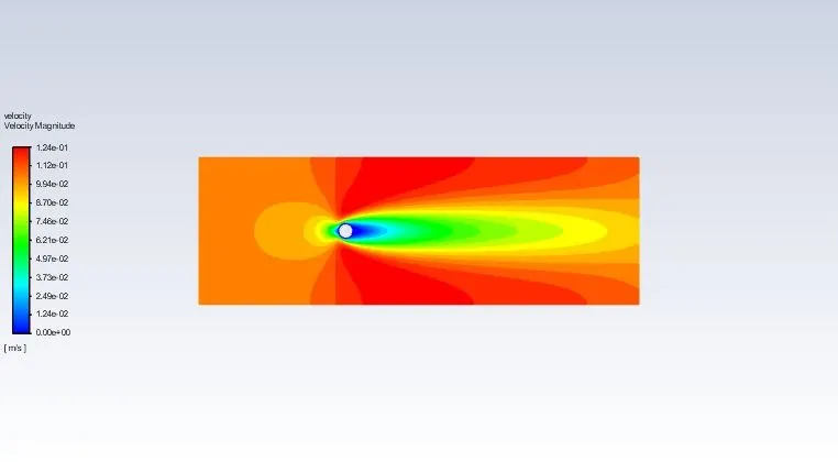
- Velocity contour
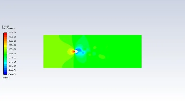
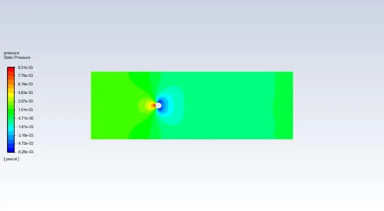
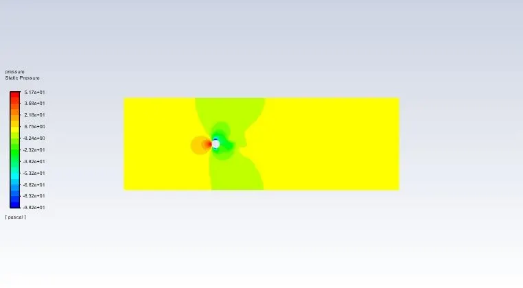
- Pressure contour
To visualize the vortex shedding, the animation is created using the velocity contour. For steady-state calculations, the number of iterations is specified and for the unsteady-state calculations, time step and time step size are mentioned. The reference values are modified for each case.
Solution:
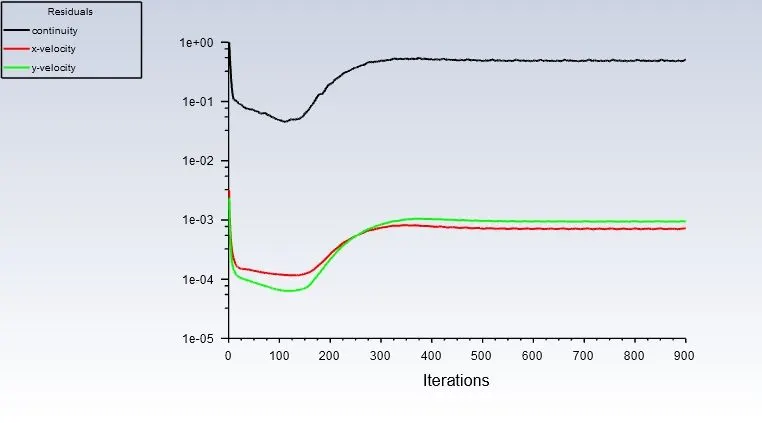
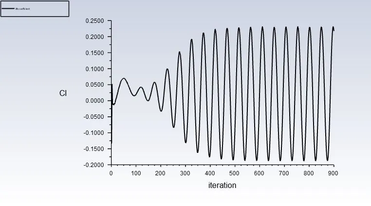
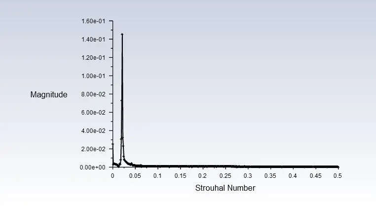
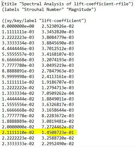
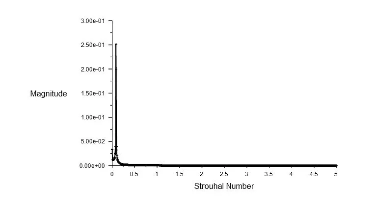
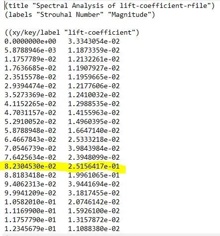
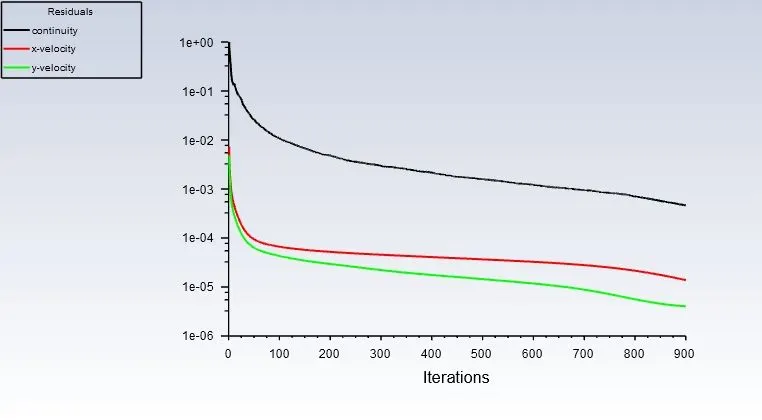
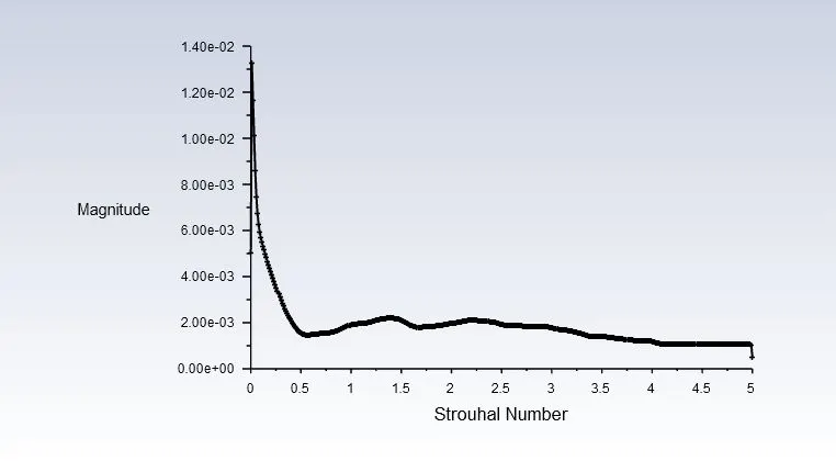
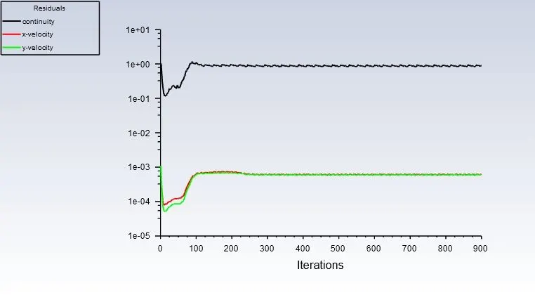
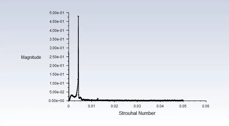
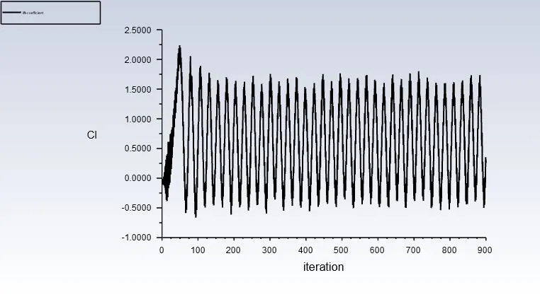
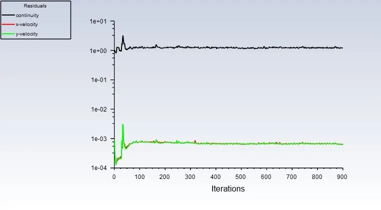
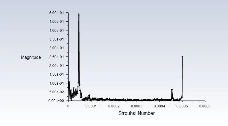
The default convergence criteria are disabled so that the simulation is performed for the desired amount of iterations. It is observed that not only the residuals plot is referred to for convergence but also the drag and lift plots are also considered to declare convergence. Once the plots are obtained, the Strouhal number can be calculated by plotting FFT based on inputs from the lift coefficient file. From the FFT plot, the value corresponding to the maximum magnitude is the Strouhal number.
Results:
PART-I:
CASE 1A: STEADY-STATE
Residuals:
Coefficient of drag:
Coefficient of lift:
Monitor point velocity:
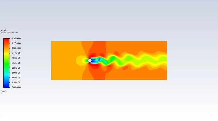
Velocity contour:
Pressure contour:
Strouhal plot:
CASE 1B: UNSTEADY-STATE
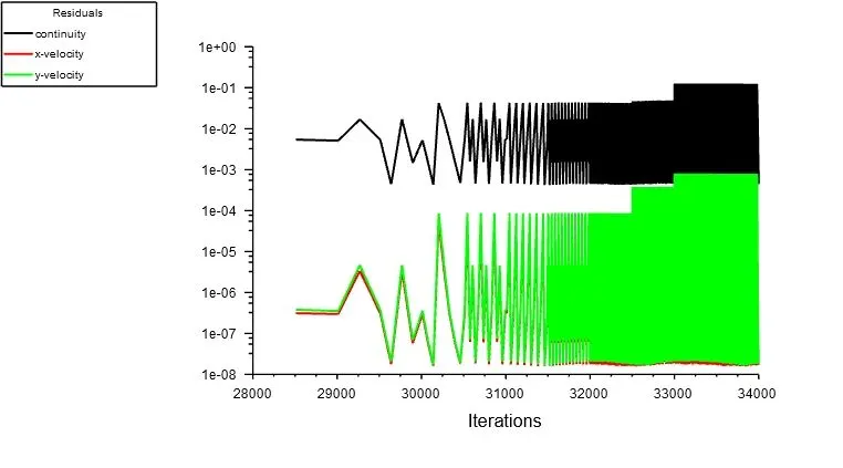
Residuals:
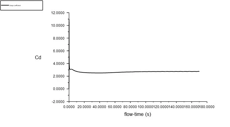
Coefficient of drag:
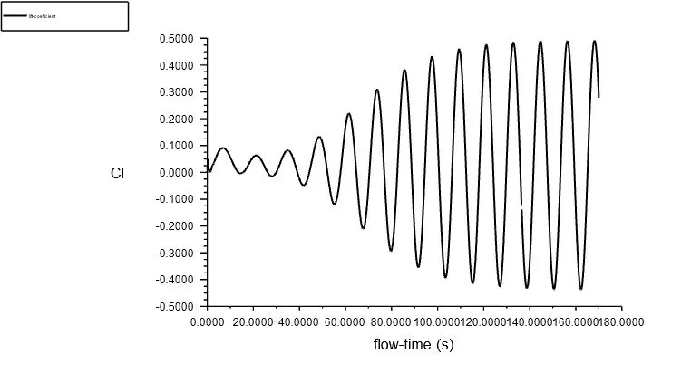
Coefficient of lift:
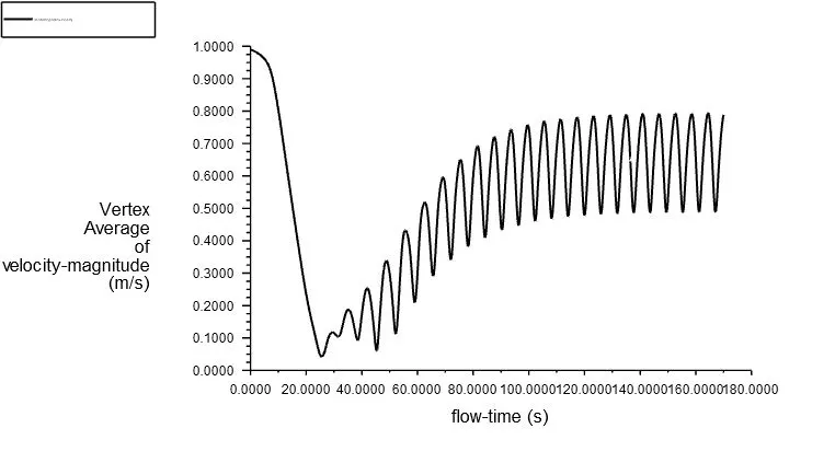
Monitor point velocity:
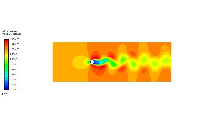
Velocity contour:
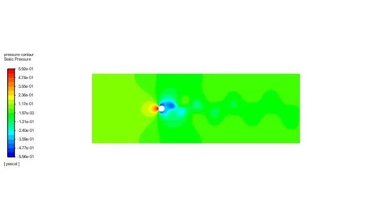
Pressure contour:
Strouhal plot:
| Case | Type | Re | V | `C_d` | `C_l` | `V_(mp)` | Sr |
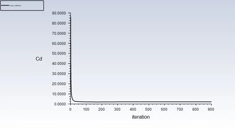
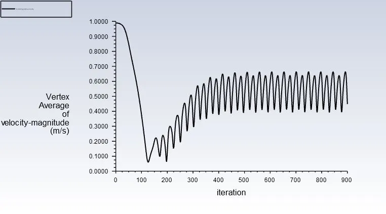
| 1a | Steady-state | 100 | 1 m/s | 2.19 | 0.217 | 0.448 m/s | 0.0211 |
| 1b | Unsteady-state | 100 | 1 m/s | 2.75 | 0.278 | 0.789 m/s | 0.0823 |
- In part-I, it is observed that even in the steady-state flow there is an unsteadiness due to the vortex shedding.
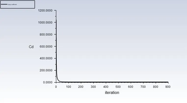
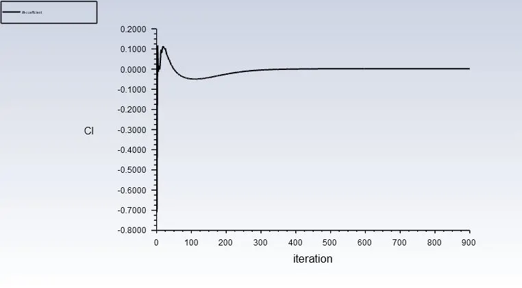
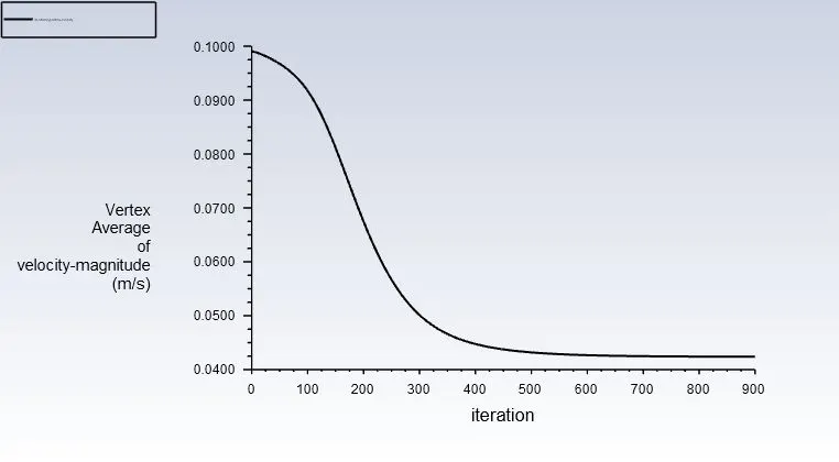
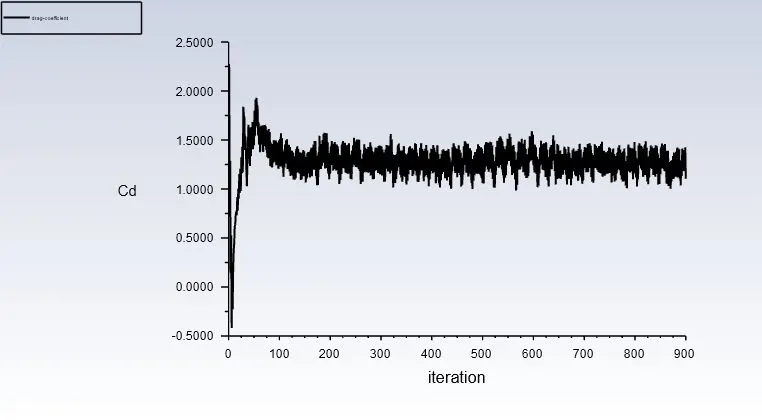
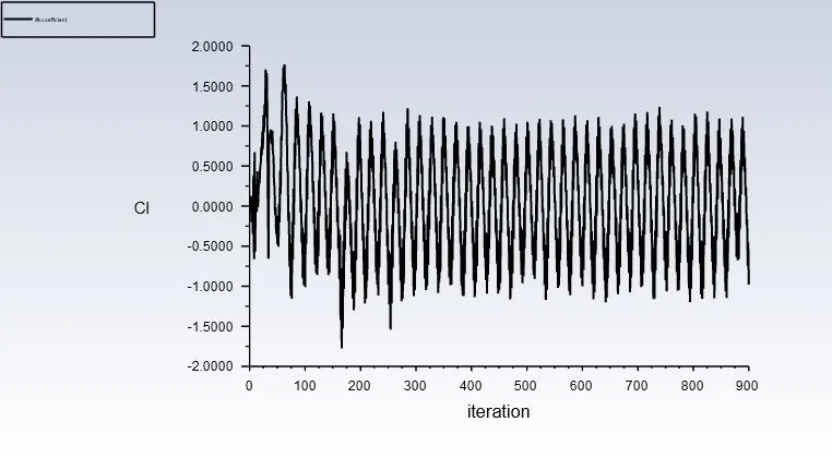
- Apart from the residuals plot, the coefficient of drag, coefficient of lift, and vertex average of monitor point velocity plots are also considered to declare convergence.
- The Strouhal number for the unsteady-state condition is higher than the steady-state indicating an increase in the unsteadiness.
PART-II:
CASE 2A: Re = 10
Residuals:
Coefficient of drag:
Coefficient of lift:
Monitor point velocity:
Velocity contour:
Pressure contour:
Strouhal plot:
CASE 2B: Re = 100
Residuals:
Coefficient of drag:
Coefficient of lift:
Monitor point velocity:
Velocity contour:
Pressure contour:
Strouhal plot:
CASE 2C: Re = 1000
Residuals:
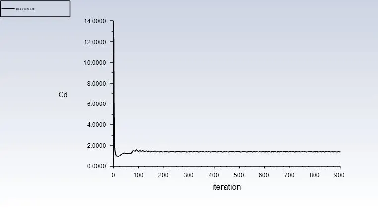
Coefficient of drag:
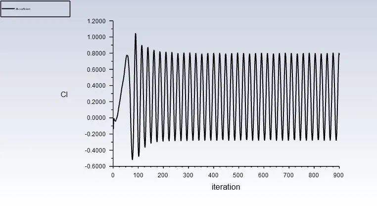
Coefficient of lift:
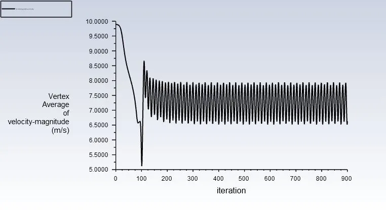
Monitor point velocity:
Velocity contour:
Pressure contour:
Strouhal plot:
CASE 2D: Re = 10000
Residuals:
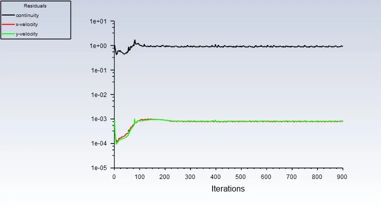
Coefficient of drag:
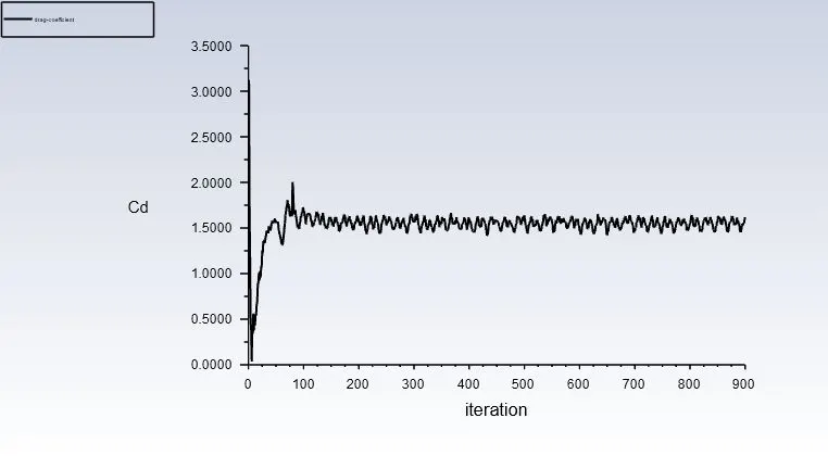
Coefficient of lift:
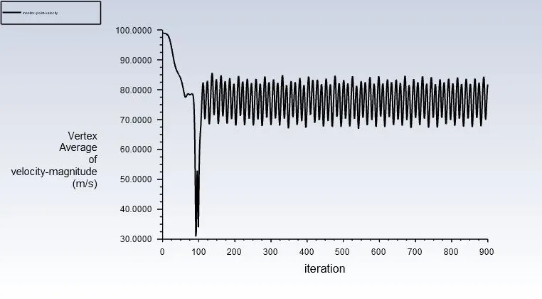
Monitor point velocity:
Velocity contour:
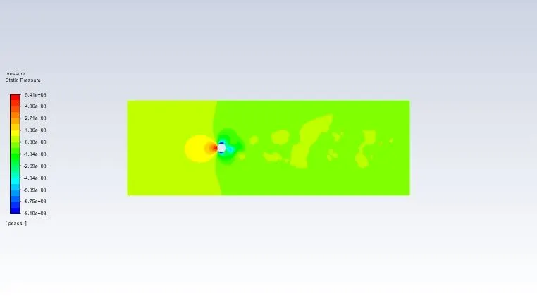
Pressure contour:
Strouhal plot:
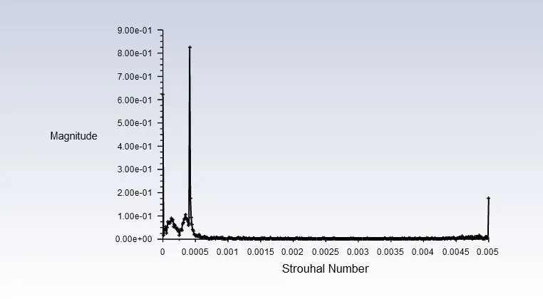
CASE 2E: Re = 100000
Residuals:
Coefficient of drag:
Coefficient of lift:
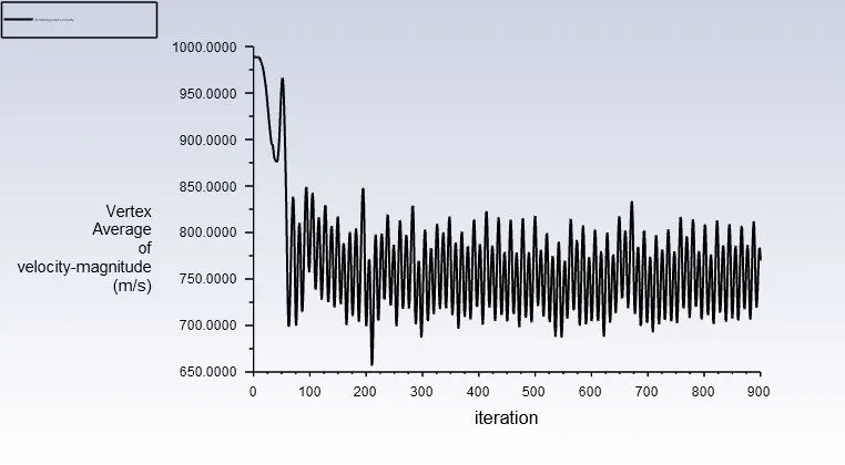
Monitor point velocity:
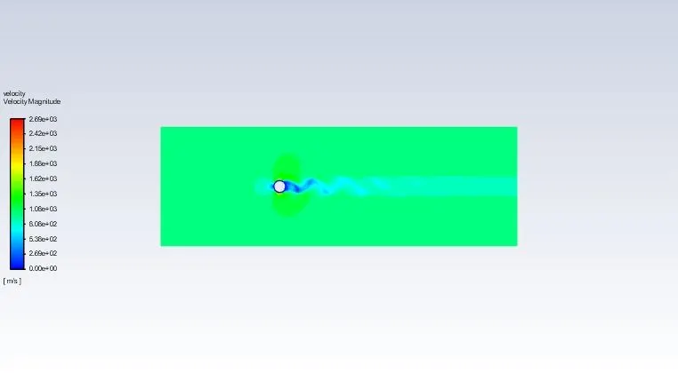
Velocity contour:
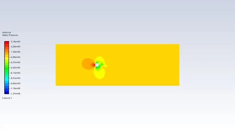
Pressure contour:
Strouhal plot:
| Case | Re | V | `C_d` | `C_l` | `V_(mp)` |
| 2a | 10 | 0.1 m/s | 6.65 | 0.002 | 0.042 m/s |
| 2b | 100 | 1 m/s | 2.19 | 0.217 | 0.448 m/s |
| 2c | 1000 | 10 m/s | 1.47 | 0.779 | 6.628 m/s |
| 2d | 10000 | 100 m/s | 1.62 | 0.259 | 81.762 m/s |
| 2e | 100000 | 1000 m/s | 1.10 | -0.979 | 769.660 m/s |
- The vortices are not formed in the first case where Re is very low (less than 40).
- In the steady-state simulation, it is observed that with an increase in Re value, there is a significant decrease in the drag coefficient.
- As the drag coefficient is inversely proportional to the velocity, the drag coefficient decreases with an increase in the velocity for a fixed frontal area and fluid properties.
VALIDATION:
For an unsteady-state flow with Re = 100, the coefficient of lift plot is compared with the one obtained from the standard reference research paper.
Figure 1: Coefficient of lift plot from reference paper
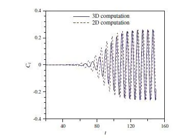
Figure 2a: Coefficient of lift plot from the present study
It is observed that the coefficient of lift reaches a steady value around 120 s in both cases. Thus the present study is valid.
CONCLUSIONS:
- The convergence of a solution depends on the steadiness of the coefficient of lift plot in addition to the residuals plot.
- The Strouhal number is higher in the case of unsteady-state flow.
- The coefficient of drag decreases with an increase in the value of Reynold's number.
REFERENCE:
B.N. Rajani, A. Kandasamy, Sekhar Majumdar, Numerical simulation of laminar flow past a circular cylinder, Applied Mathematical Modelling, Volume 33, Issue 3, 2009