Rayleigh Taylor Instability Challenge
Introduction:
Rayleigh–Taylor instability is the instability of an interface between two fluids of different densities which occurs when the lighter fluid is pushing the heavier fluid. Water suspended atop oil is an everyday example of Rayleigh–Taylor instability, and it may be modeled by two completely plane-parallel layers of immiscible fluid, the denser on top of the less dense one and both subject to the Earth's gravity. The equilibrium here is unstable to any perturbations or disturbances of the interface: if a parcel of heavier fluid is displaced downward with an equal volume of lighter fluid displaced upwards, the potential energy of the configuration is lower than the initial state. Thus, the disturbance will grow and lead to a further release of potential energy, as the denser material moves down under the (effective) gravitational field, and the less dense material is further displaced upwards. This was the set-up as studied by Lord Rayleigh. The important insight by G. I. Taylor was his realization that this situation is equivalent to the situation when the fluids are accelerated, with the less dense fluid accelerating into the denser fluid. This occurs deep underwater on the surface of an expanding bubble and in a nuclear explosion.
Practical CFD models that have been based on the mathematical analysis of Rayleigh Taylor waves:
- Richtmyer–Meshkov instability (RMI)
Richtmyer–Meshkov instability occurs when two fluids of different density are impulsively accelerated. Normally this is by the passage of a Shock Wave. The development of the instability begins with small amplitude perturbations which initially grow linearly with time. This is followed by a nonlinear regime with bubbles appearing in the case of a light fluid penetrating a heavy fluid, and with spikes appearing in the case of a heavy fluid penetrating a light fluid. A chaotic regime eventually is reached and the two fluids mix. This instability can be considered the impulsive-acceleration limit of the Rayleigh–Taylor instability.
- Kelvin–Helmholtz instability
The Kelvin–Helmholtz instability typically occurs when there is velocity shear in a single continuous fluid, or additionally where there is a velocity difference across the interface between two fluids.
- Plateau–Rayleigh instability,
The Plateau–Rayleigh instability, often just called the Rayleigh instability, explains why and how a falling stream of fluid breaks up into smaller packets with the same volume but less surface area. It is related to the Rayleigh–Taylor instability and is part of a greater branch of fluid dynamics concerned with fluid thread breakup. This fluid instability is exploited in the design of a particular type of inkjet technology whereby a jet of liquid is perturbed into a steady stream of droplets.
The driving force of the Plateau–Rayleigh instability is that liquids, by virtue of their surface tensions, tend to minimize their surface area. A considerable amount of work has been done recently on the final pinching profile by attacking it with self-similar solutions.
Methodology:
1.Geometry:
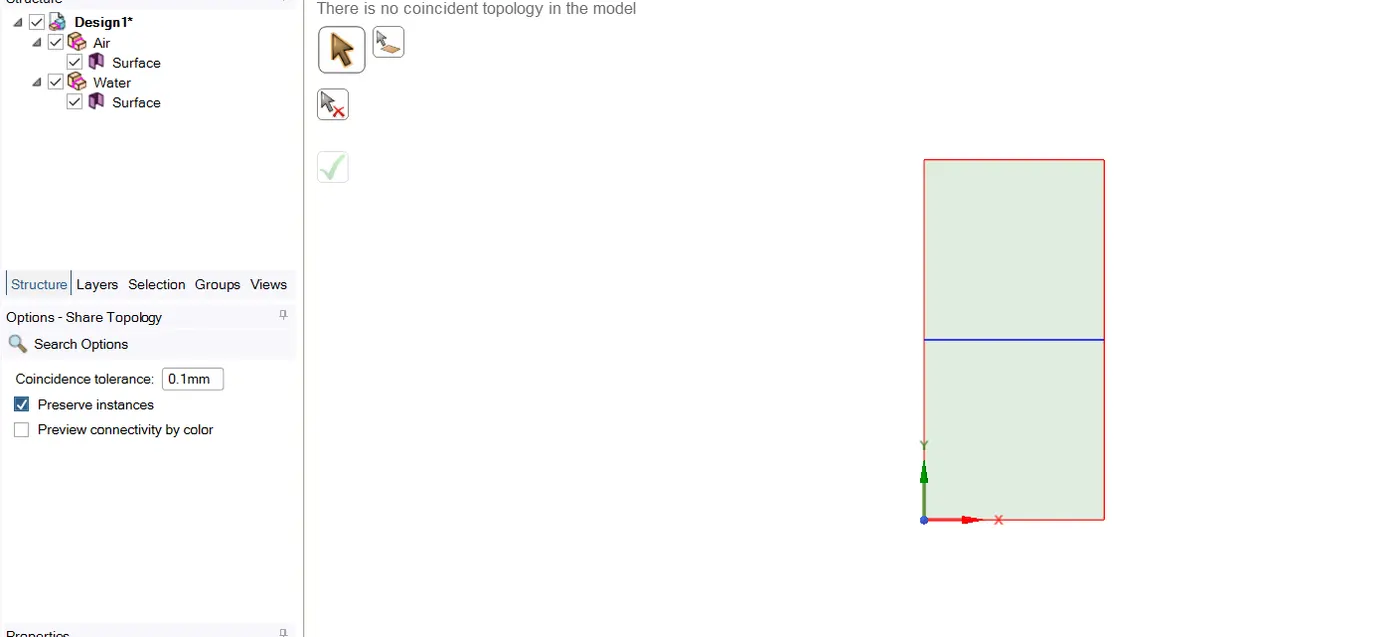
The required geometry was created in Spaceclaim. Two square surfaces of the 20*20 mm dimension were created one above the other in 2D as shown in the figure below. In order to have a conformal mesh, share topology was set to share.
2.Meshing:
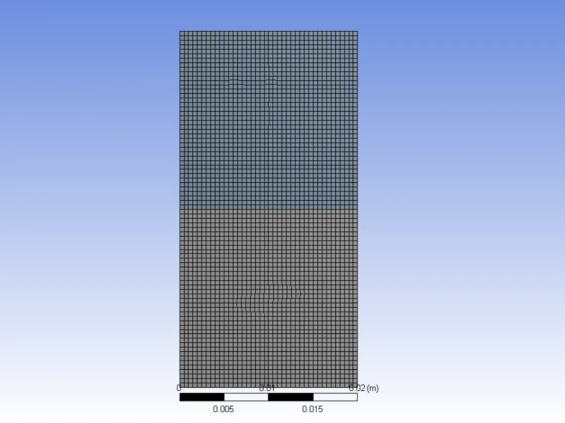
Case1 (Baseline Mesh):
Element size: 0.5mm
Nodes: 3321
Elements: 3200
Mesh Metric: Element Quality
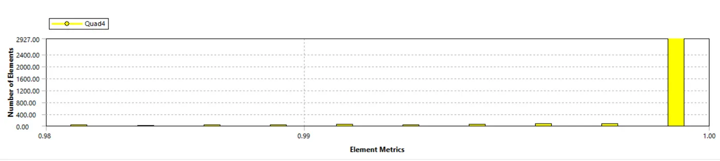
The mesh metric that identifies the elements according to their quality was employed and it can be seen that the elements of the lowest quality are minimal, most of the elements have very high quality.
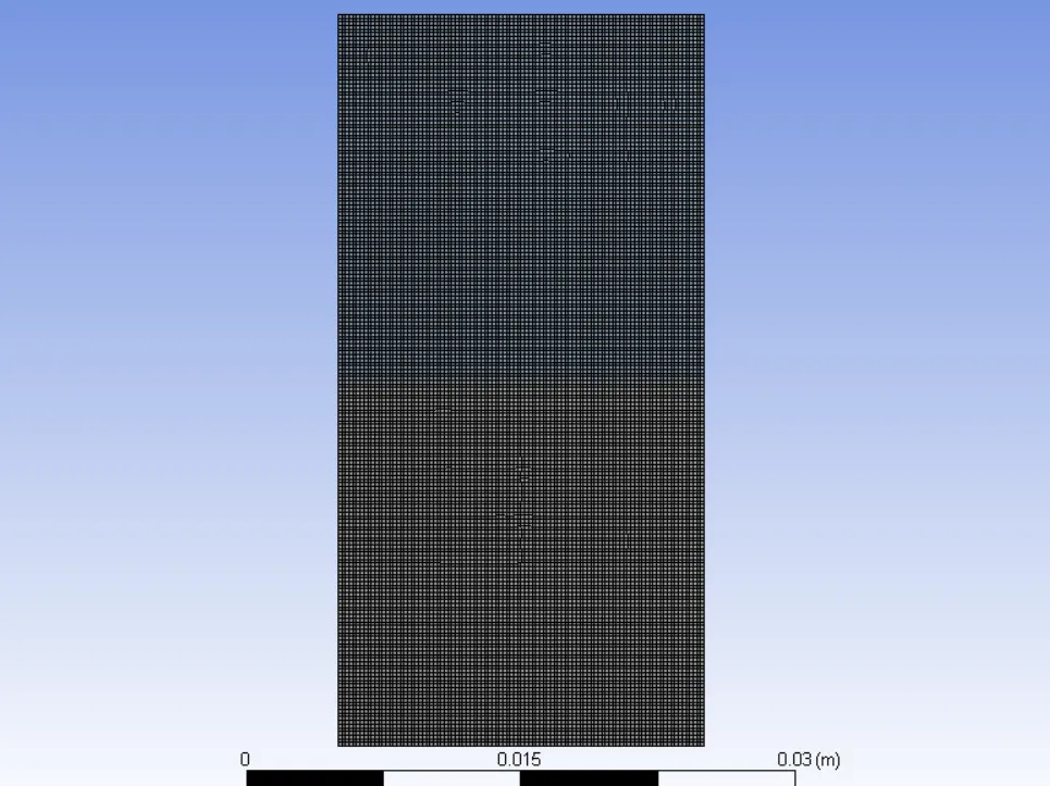
Case 2:
Element size: 0.2mm
Nodes: 20301
Elements: 20000
Mesh Metric: Element Quality
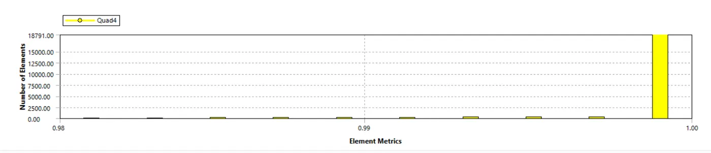
The mesh metric that identifies the elements according to their quality was employed and it can be seen that the elements of the lowest quality are minimal, most of the elements have very high quality.
3.Setup and Results:
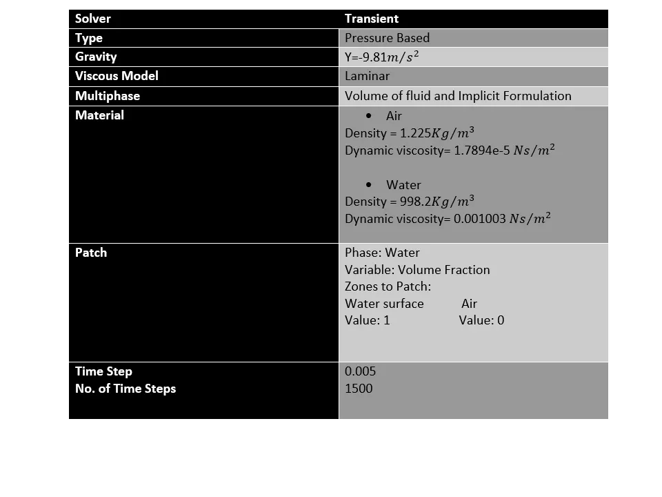
Case 1:
Residual Plot:
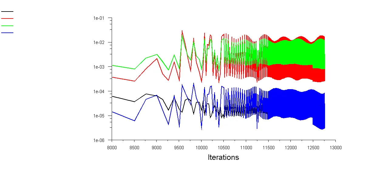
Animation:
Case 2:
Residual Plot:
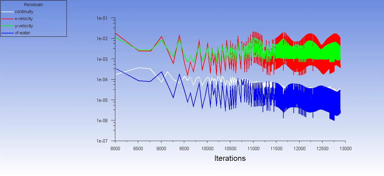
Animation:
Case 3:
Element size: 0.25mm
Nodes: 13041
Elements: 12800
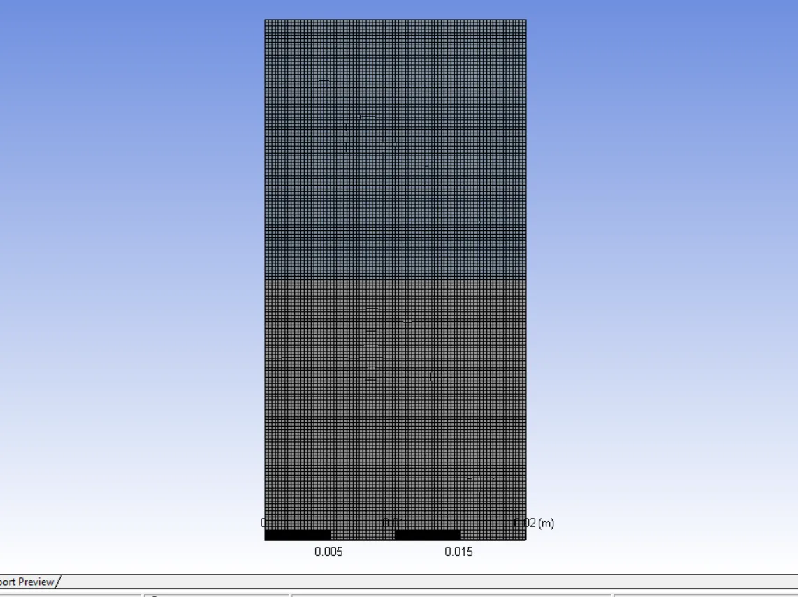
Mesh Metric: Element Quality
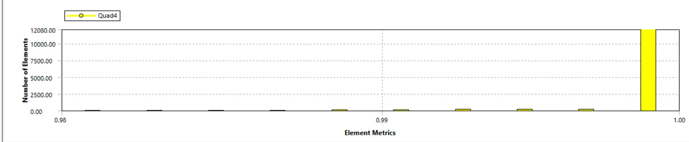
The mesh metric that identifies the elements according to their quality was employed and it can be seen that the elements of the lowest quality are minimal, most of the elements have very high quality.
Simulation:
Materials:
Water:
Density = 998.2 Kg/m^3
Dynamic viscosity= 0.001003 Kg-m/s
User-defined Material:
Density = 400 Kg/m^3
Dynamic viscosity= 0.001 Kg-m/s
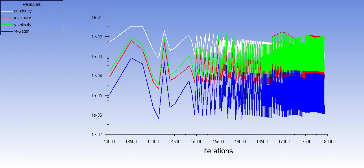
Residual plot:
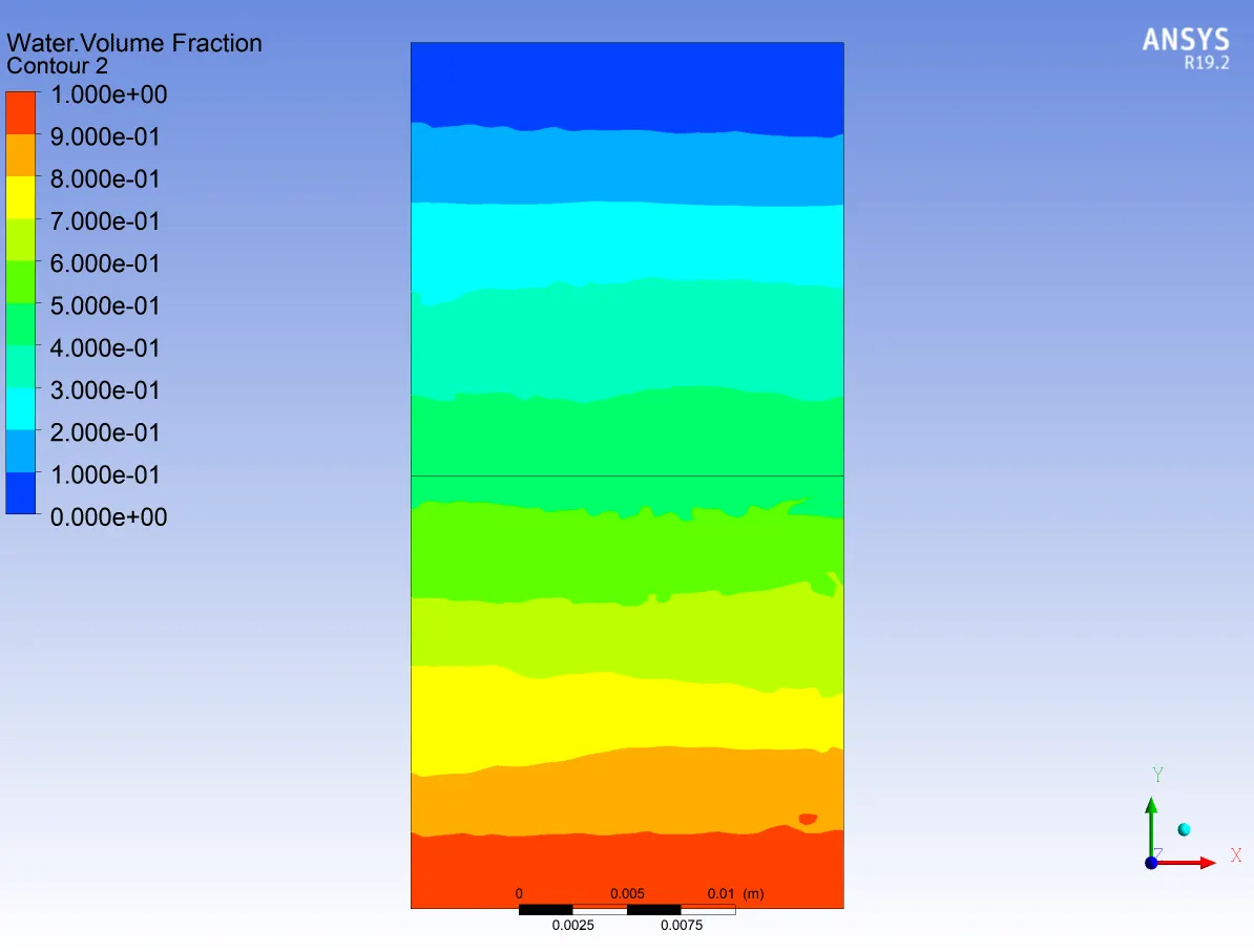
Contour Plots at different time steps:
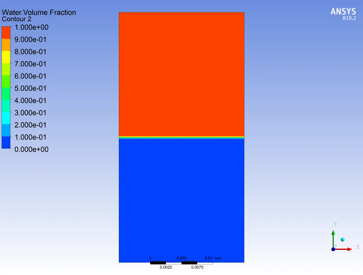
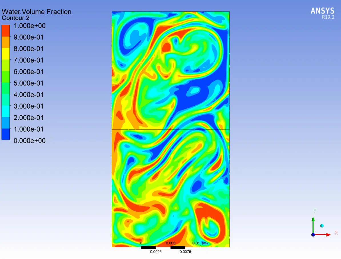
Timestep=0 Timestep=200
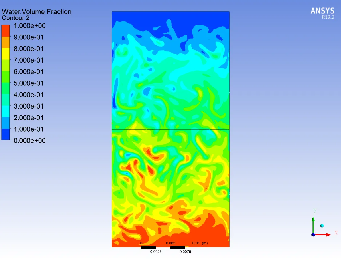
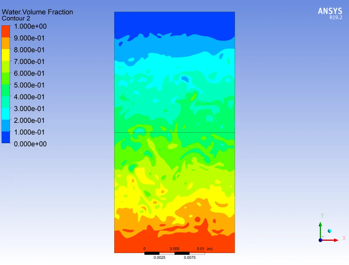
Timestep=400 Timestep= 600
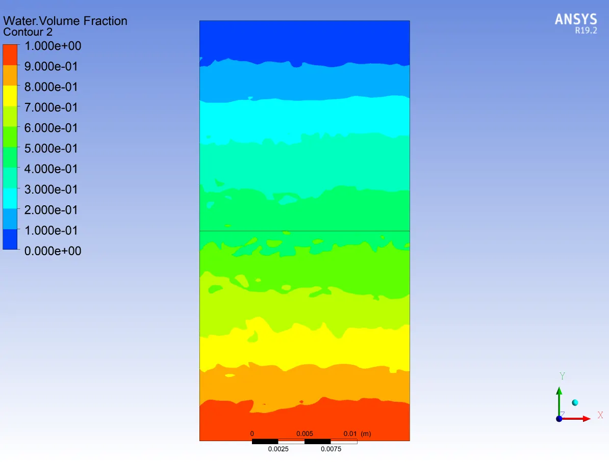
Timestep=800 Timestep=1000
Animation:
Effect of mesh size on simulation:
From the above simulation results of two cases, we can observe that initially the simulation starts with the state of hydrostatic equilibrium and the Rayleigh Taylor instability is observed at the interface when the fluid with lower density (i.e. Air) pushes the higher density fluid (i.e. Water).
Due to this shock wave formation at the interface takes place. The formation of bubbles starts taking place, which compresses the heavy fluid around it. Due to this formation of shock waves of multidimensional fashion generates and it gets stronger and stronger as it moves upwards.
By refining the mesh, Simulation results got smoother at the irregularities that take place at the interface of the two fluids. As higher density fluid replaces the lower density fluid, the formation of air bubbles and vortex takes place. The lower density fluid travels towards the upward region with the time. In the result animation, we can observe the formation of waves and the bubbles that get rapped at the lower region during the initial stage and then they travel towards the upward region generating shock waves. At the end of the simulation, we observe that the two phases get separated from each other and the water settles below the air. Some diffusivity between them which is a volume fraction of air and water can be observed.
why a steady-state approach might not be suitable for these types of simulation?
As we know the steady-state analysis is independent of time and also the steady-state analysis is used in CFD to study the end results of the fluid behavior. But we are interested in studying the instability from the start till the end where a steady-state is reached. In this project, we want to study the instability at the interface from the instant the instability starts occurring. Therefore, the steady-state approach might not be suitable for these types of simulation.
Atwood Number:
The Atwood number is a dimensionless number in fluid dynamics used in the study of hydrodynamic instabilities in density stratified flows. It is a dimensionless density ratio related to the density of the heavier fluid and the density of the lighter fluid. (The difference in the fluid densities divided by their sum). Atwood number is an important parameter in the study of Rayleigh–Taylor instability.
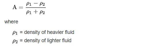
In our case:
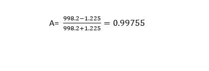
As we know,
For Atwood number close to 0, RT instability flows take the form of symmetric “fingers” of fluid.
for Atwood number close to 1, the much lighter fluid “below” the heavier fluid takes the form of larger bubble-like plumes.
Therefore, From the simulations, we can observe the formation of waves and the bubbles that get rapped at the lower region during the initial stage and then they travel towards the upward region generating shock waves. These smaller bubbles join with other small bubbles resulting in a larger bubble. The Atwood number value we obtained was close to 1. Thus, the results can be validated by calculating the value of Atwood's number.