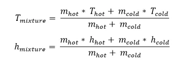
Mixing efficiency

Mixing Tee simulation: Comparison of mixing effectiveness

Aim:

To set up steady-state simulations to compare the mixing effectiveness of a short and long mixing tee for different momentum ratio.

Introduction :

Tee joints are important flow control devices, in which two fluid streams with different physical and chemical properties mix together. It is called Tee joint because it splits the flow and the angle between them is 90 degree. When there is a large temperature difference between the two streams, if proper design steps are not taken then large metal temperature fluctuations can occur in the region where the two streams meet, And the fluid may leak due to through-wall cracking. It is therefore important to make sure that the temperature fluctuations are such that the piping system can withstand them. Options can include improving the mixing of the two streams to reduce the temperature fluctuations through redesign of the piping system such that the momentum ratio of the two fluid streams is favourable to rapid mixing.

The steady-state simulations are carried using ANSYS Fluent for short and long mixing tee for different momentum ratio. Once the simulation is complete then the mixing effectiveness of a short and long mixing tee is compared.

Application: Mixing tees are widely used in the petrochemical industry, Air conditioning system etc.

Momentum ratio = velocity at cold inlet / velocity at hot inlet

Methodology :

1.Modelling:

The mixing tee configurations was modelled in SpaceClaim.SpaceClaim offers a feature to create a Fluid Volume using the Volume Extract option to distinguish the volume through which the fluid flow will occur against the entire model. This feature removes the thickness associated with these models and is not required as part of the scope of this challenge as they are solid structures on which there is no analysis being performed such as thermal conductivity.

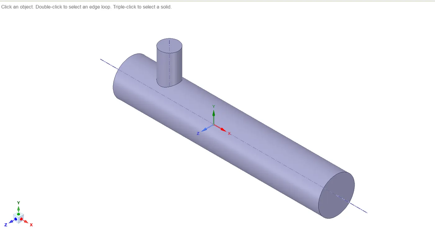
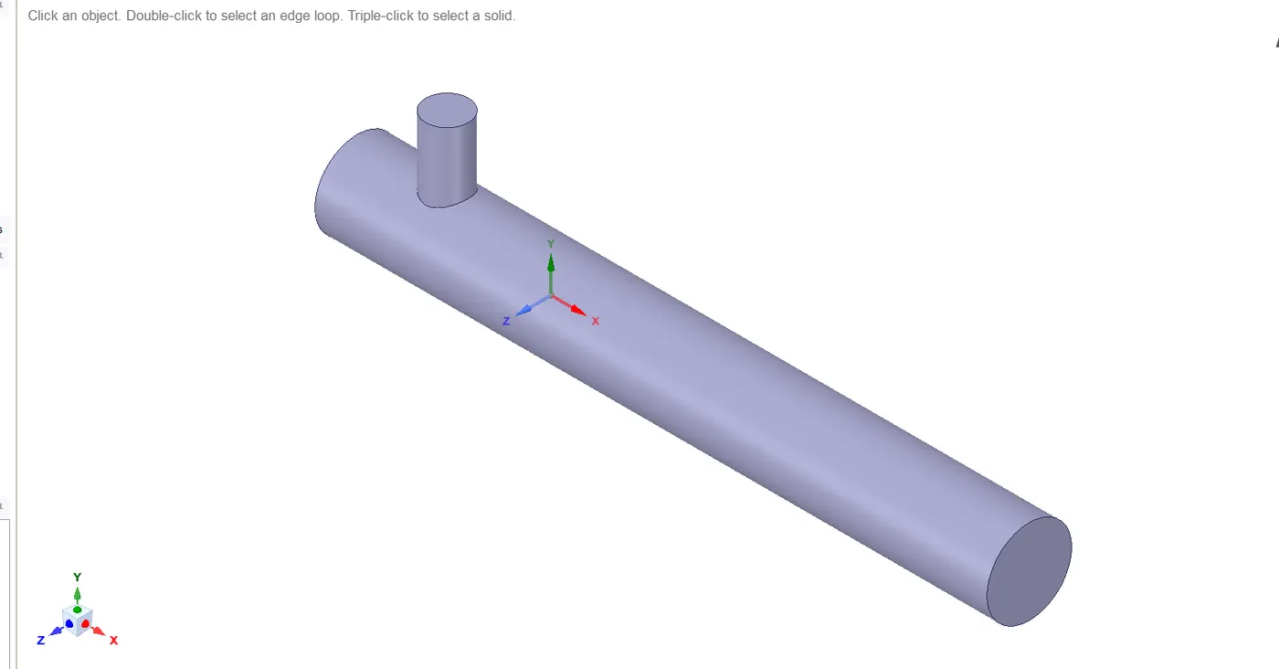
Short mixing tee Long mixing tee

-----------------------------------------------------------------------------------------------------------------------------------------------------------------------------------------------------------------------------------------------------------------------

2.Meshing:

Meshing is the important part to get the accurate results of the experiment, it is an integral part of the engineering simulation process where complex geometries are divided into simple elements that can be used as discrete local approximations of the larger domain. The mesh influences the accuracy, convergence and speed of the simulation. The model is meshed using ANSYS mesher.

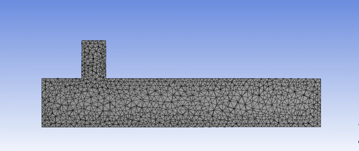
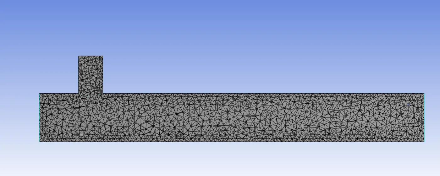
Short mixing tee with a mesh element size of 3mm long mixing tee with a mesh element size of 3mm

----------------------------------------------------------------------------------------------------------------------------------------------------------------------------------------------------------------------------------------------------------------------

3.Simulation and results:

The simulations were performed using the ANSYS Fluent; the solver tries to solve the Navier Stokes Equation. There are two different types of flow, laminar and turbulent. Laminar flow is smooth where the adjacent layers of fluid will undergo sliding between each other. The turbulent is chaotic and random. It is normally unsteady, dissipative and 3 dimensional. Reynolds number decides whether the flow is laminar or turbulent. For our project, we take the flow to be turbulent.

There are different methods to solve the flow. The most common of those are

• Direct Numerical Simulation (DNS) – It solves the Navier-stokes equation numerically. It requires a very fine grid size and requires very high computer memo It can solve all turbulence scales.
• Reynolds Averaged Navier-Strokes Equation (RANS) – It gives the approximate time-averaged solution to the Navier-Stokes equation. The velocity field is fluctuating and it cannot solve all turbulence scales.
• Large-eddy simulation (LES): It solves the large eddies. The simulation is time-dependent.

As of today majority of engineering simulations are RANS based. In terms of speed RANS based simulation is much quicker. The steady RANS equation with k-epsilon and k-omega SST model is used for the first case.

Case 1: Short mixing tee

1. K-epsilon (k-ε) model with momentum ratio 2 :

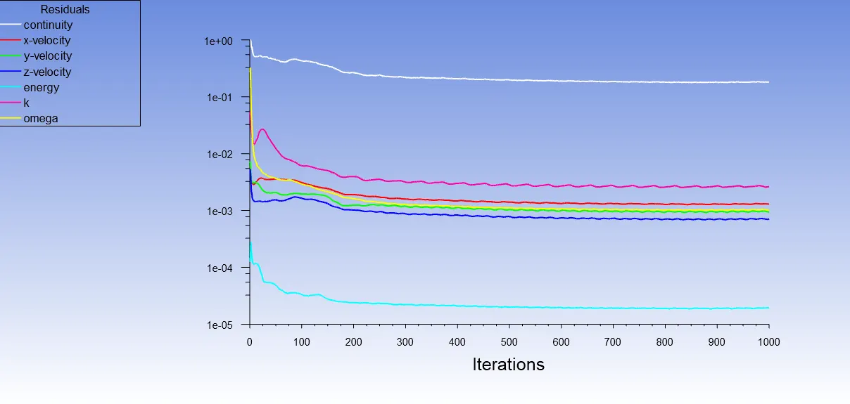
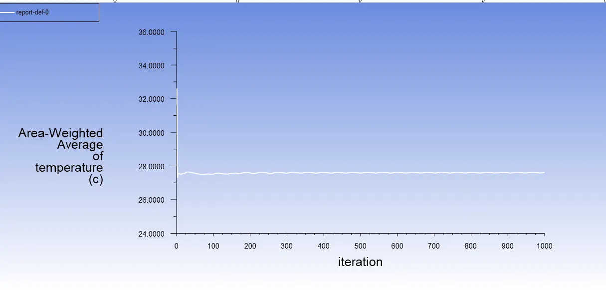
convergence plot	Area weighted average(°C) plot
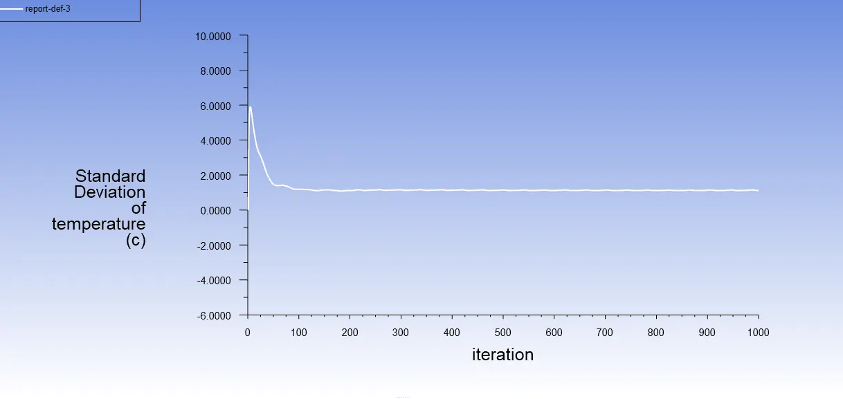
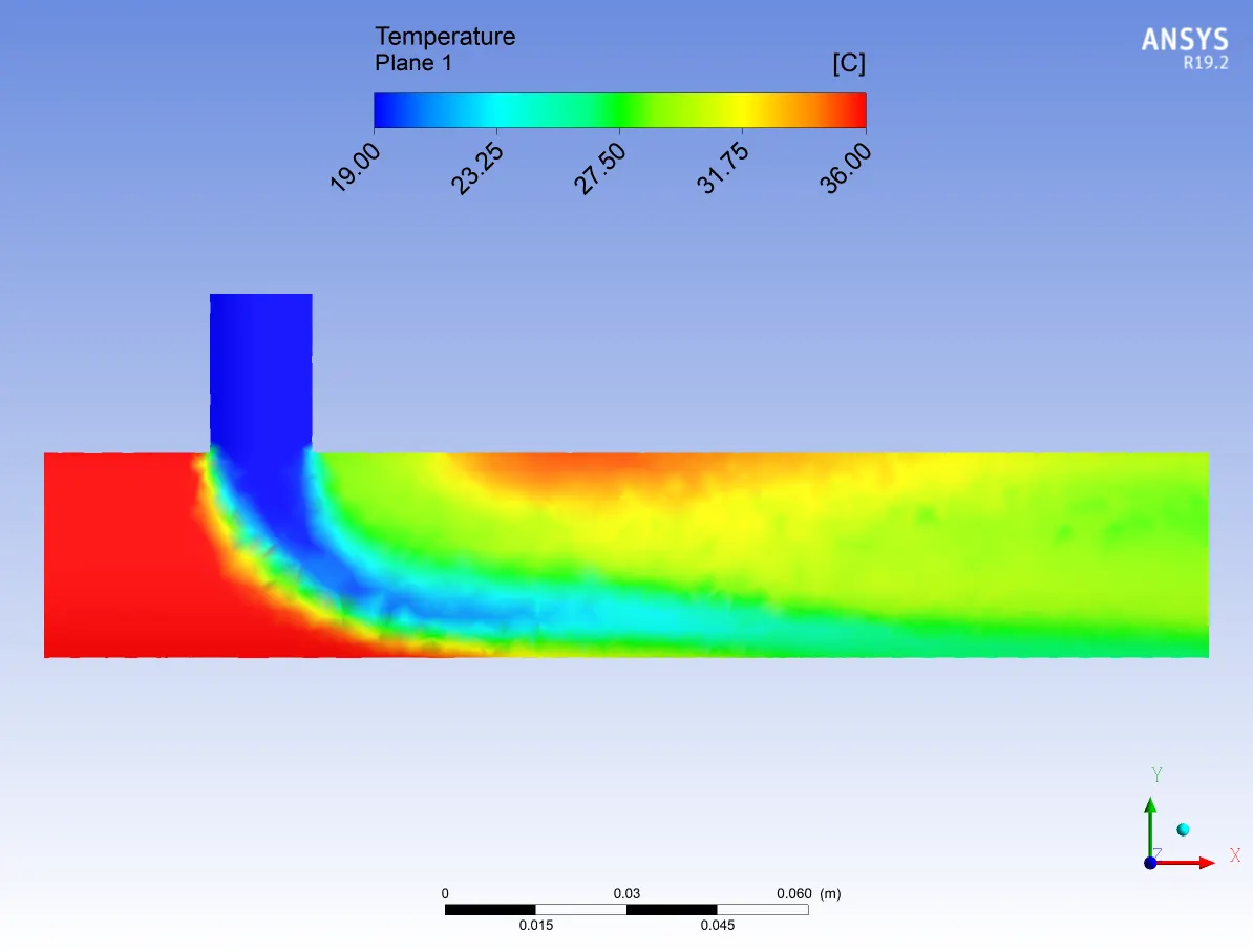
Standard deviation of temperature(°C) Plot	Temperature contour plot along the pipe
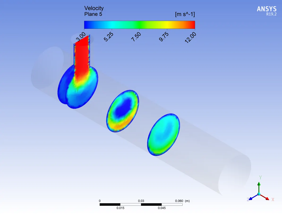
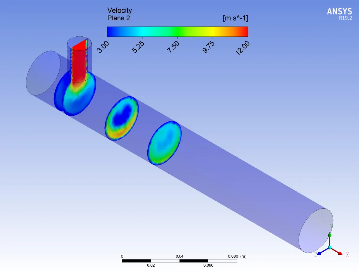
Temperature contour plot across the pipe	Velocity contour plot along the pipe
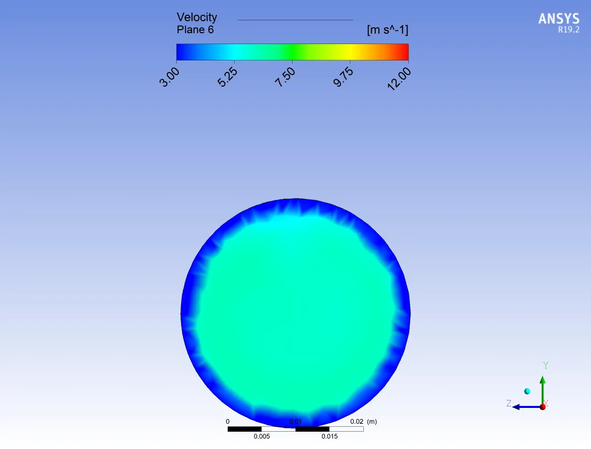
Velocity contour plot across the pipe	Temperature line plot along the length of the pipe
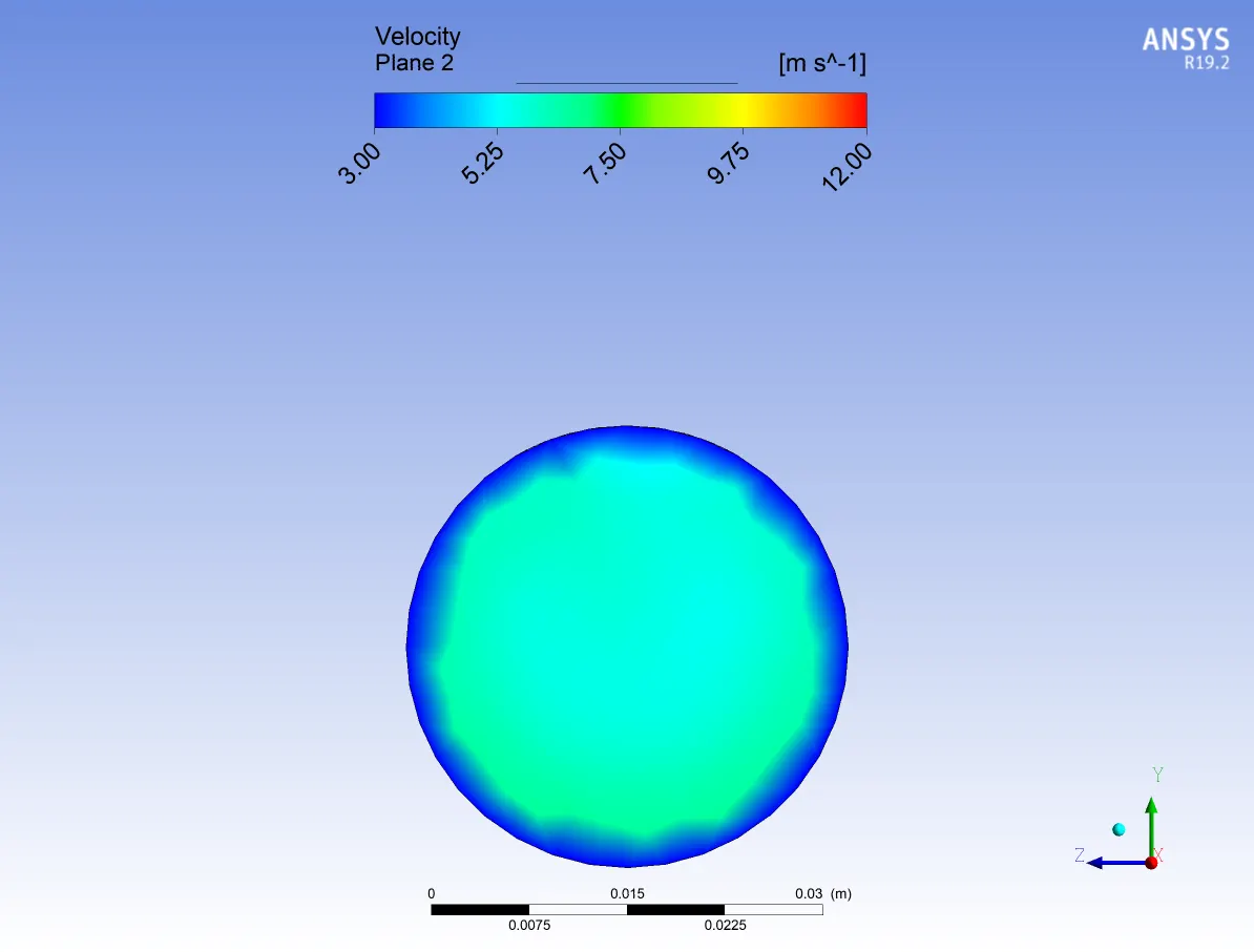
Velocity line plot along the length of the pipe	Temperature and Velocity contour plot at the outlet
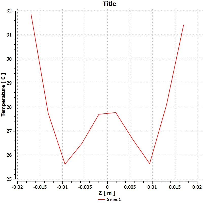
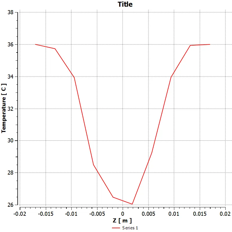
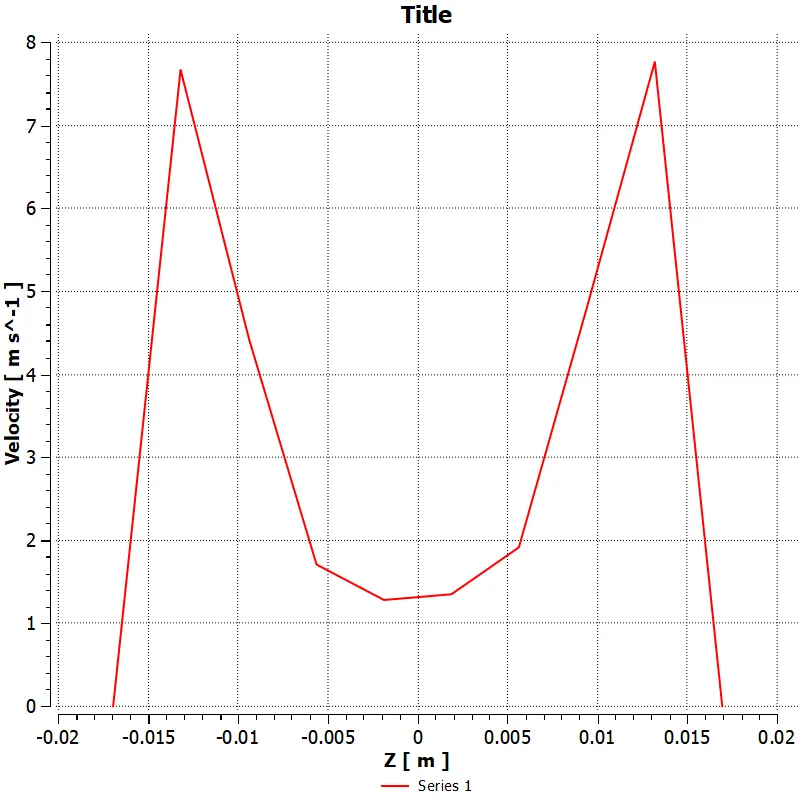
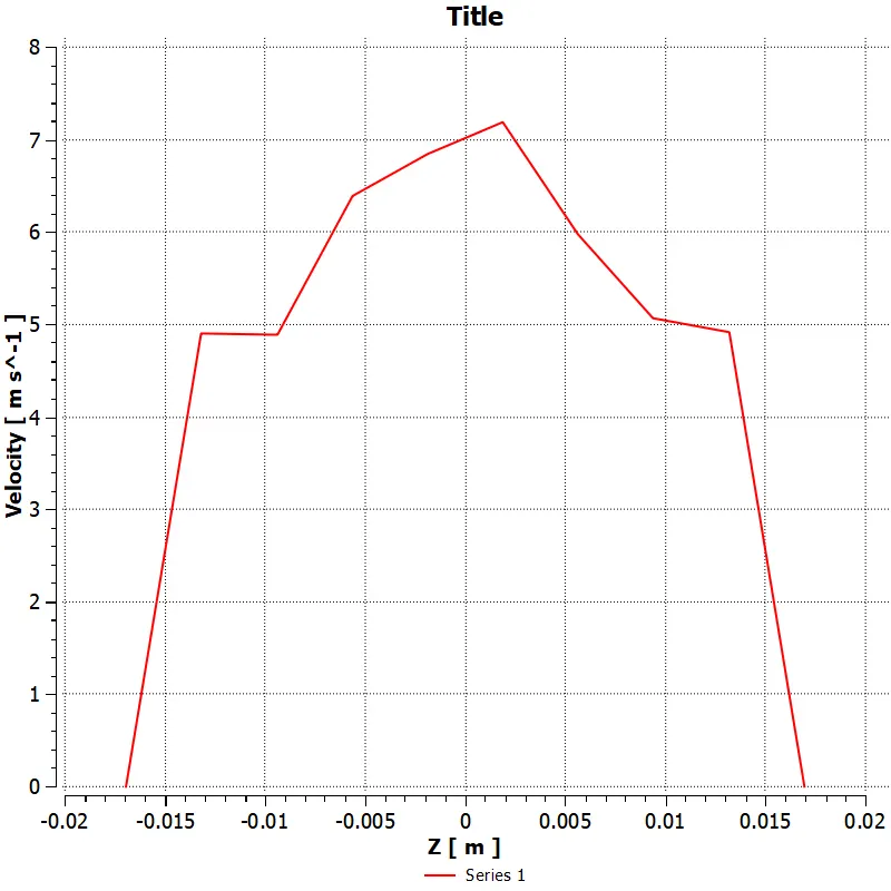
Temperature line plot across the length of the pipe	Velocity line plot across the length of the pipe

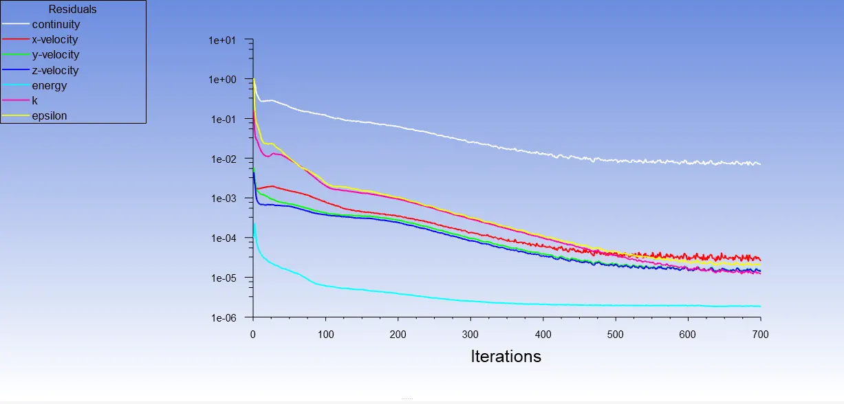
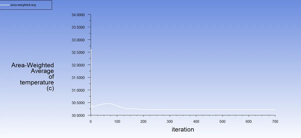
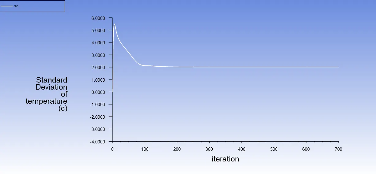
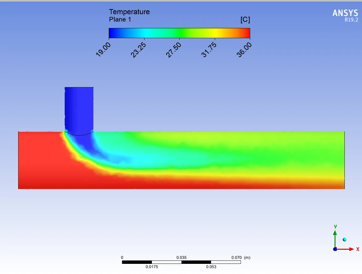
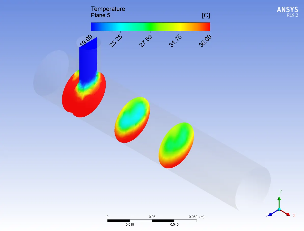
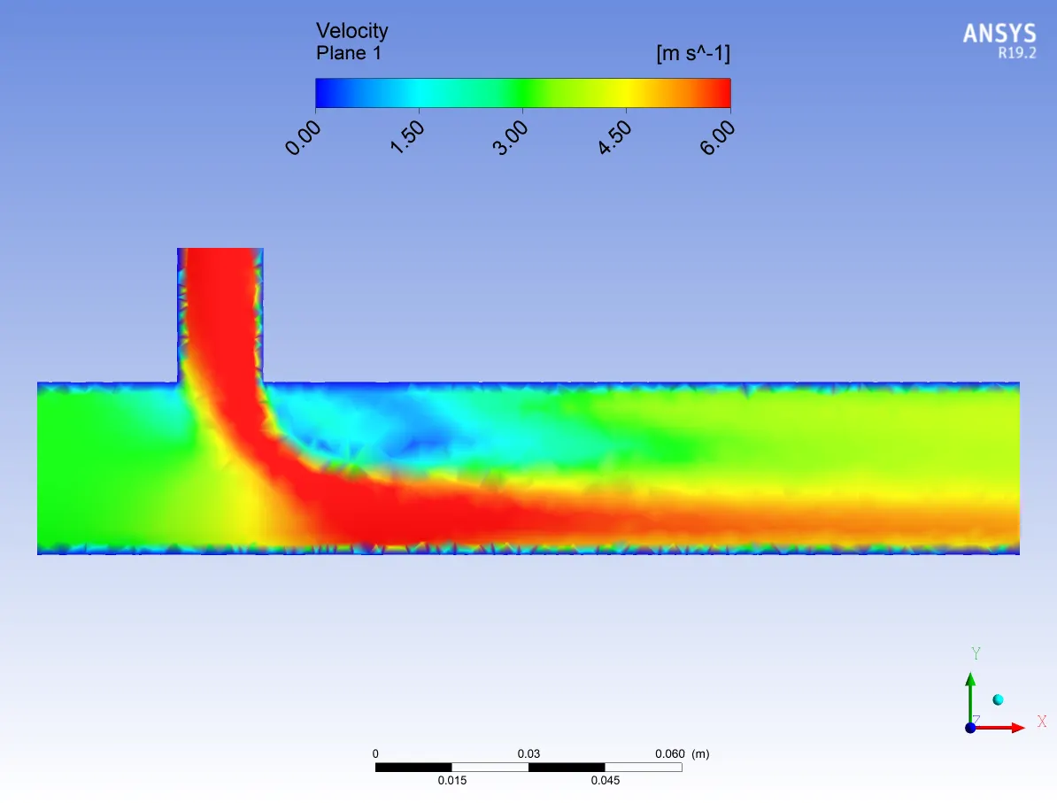
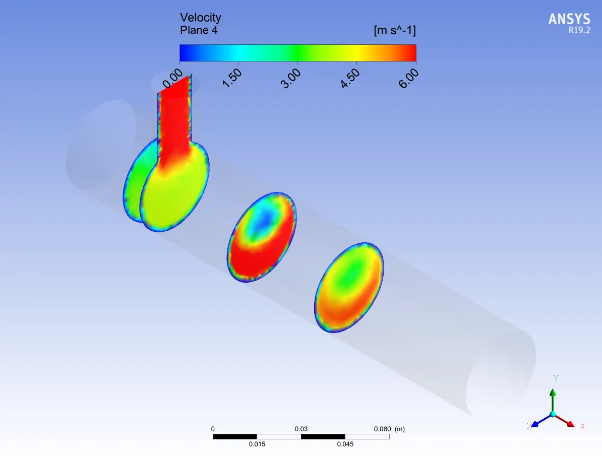
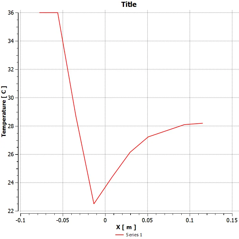
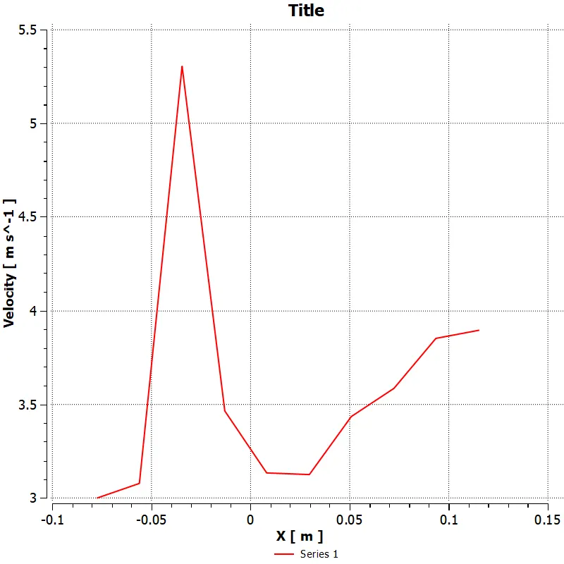
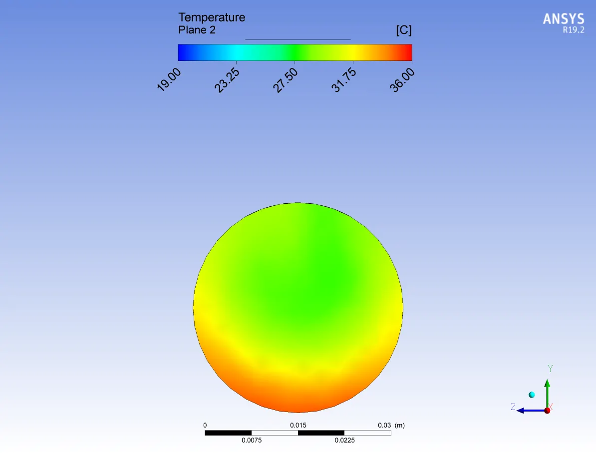
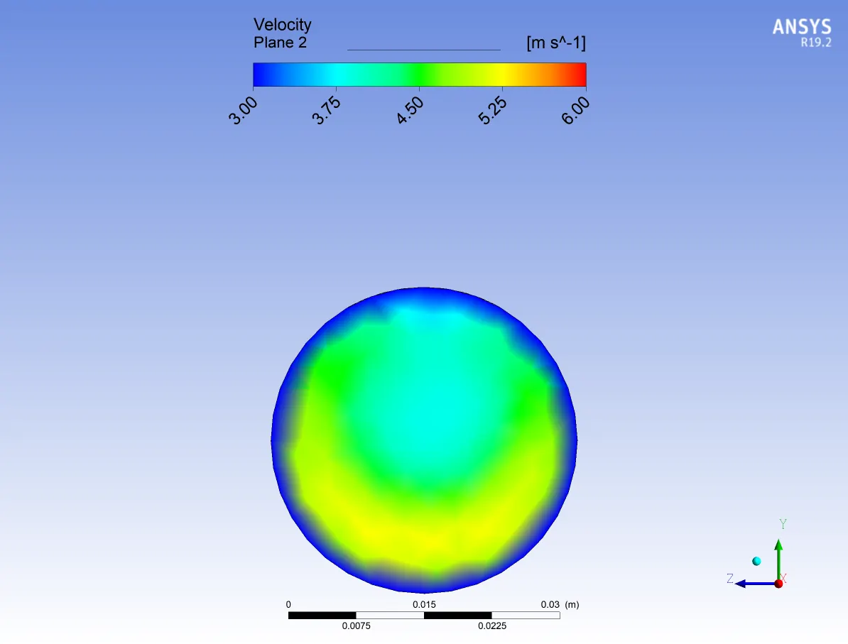
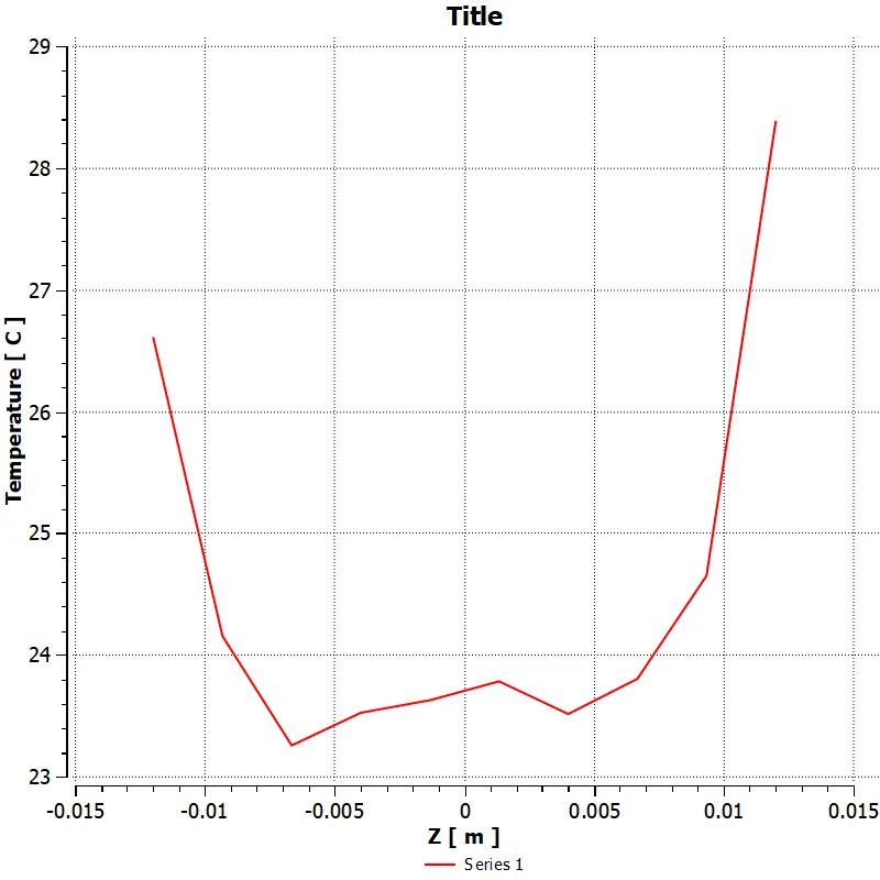
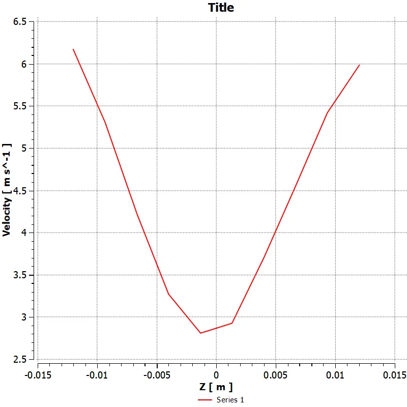
2. K-epsilon (k-ε) model with momentum ratio 4 :

convergence plot	Area weighted average(°C) plot
Standard deviation of temperature(°C) Plot	Temperature contour plot along the pipe
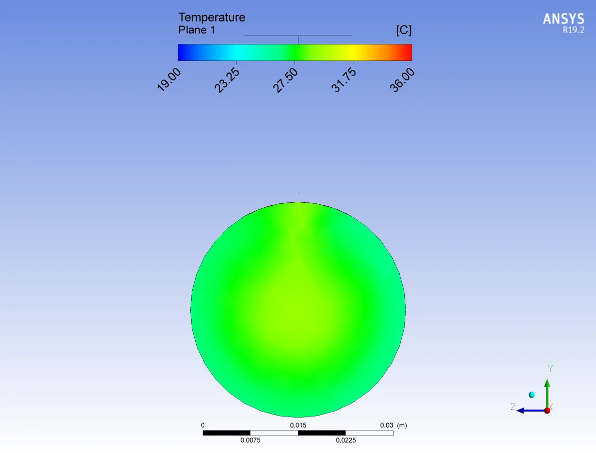
Temperature contour plot across the pipe	Velocity contour plot along the pipe
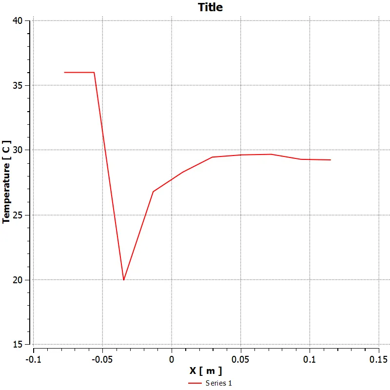
Velocity contour plot across the pipe	Temperature line plot along the length of the pipe
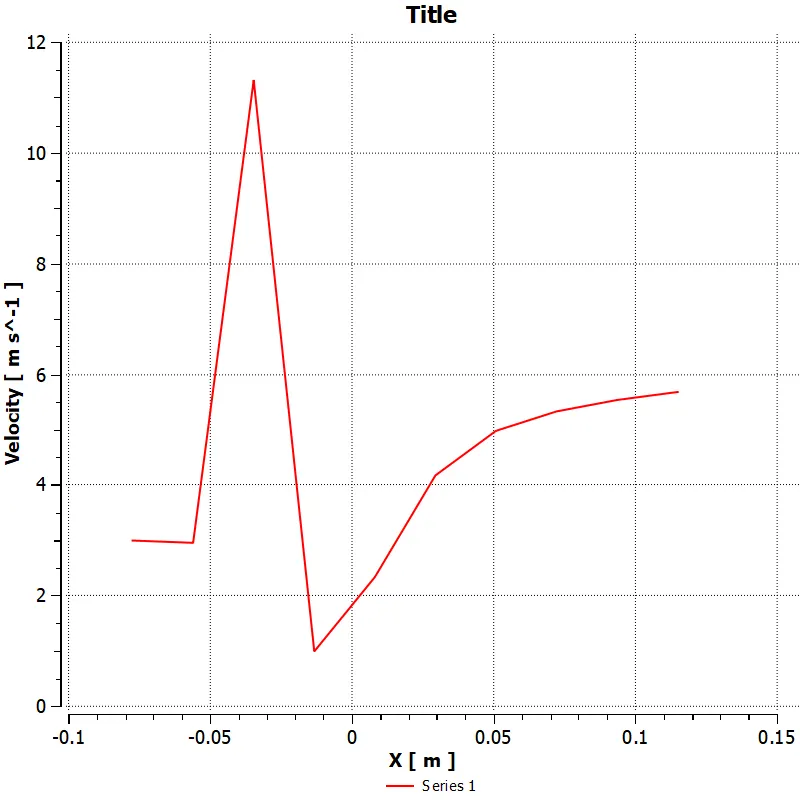
Velocity line plot along the length of the pipe	Temperature and Velocity contour plot at the outlet
Temperature line plot across the length of the pipe	Velocity line plot across the length of the pipe

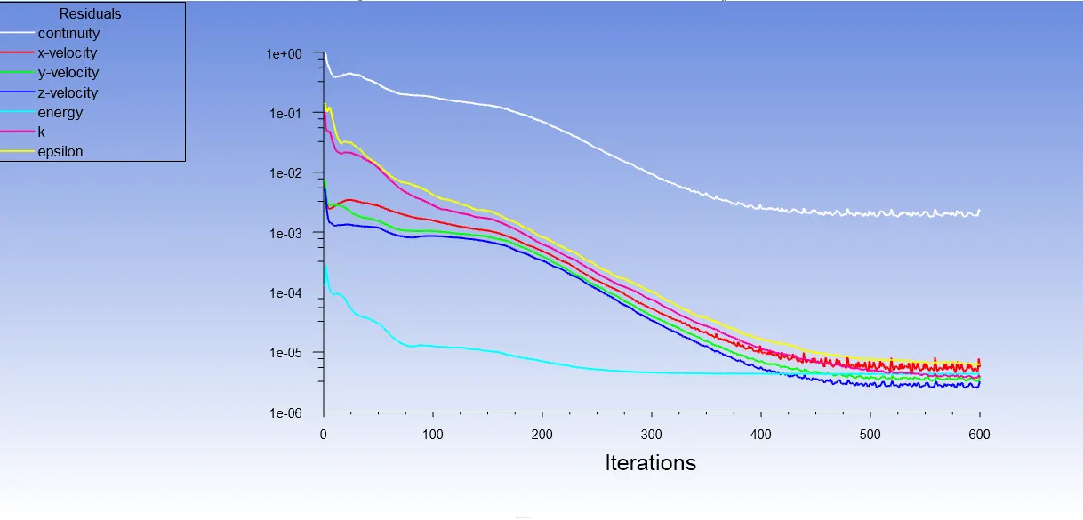
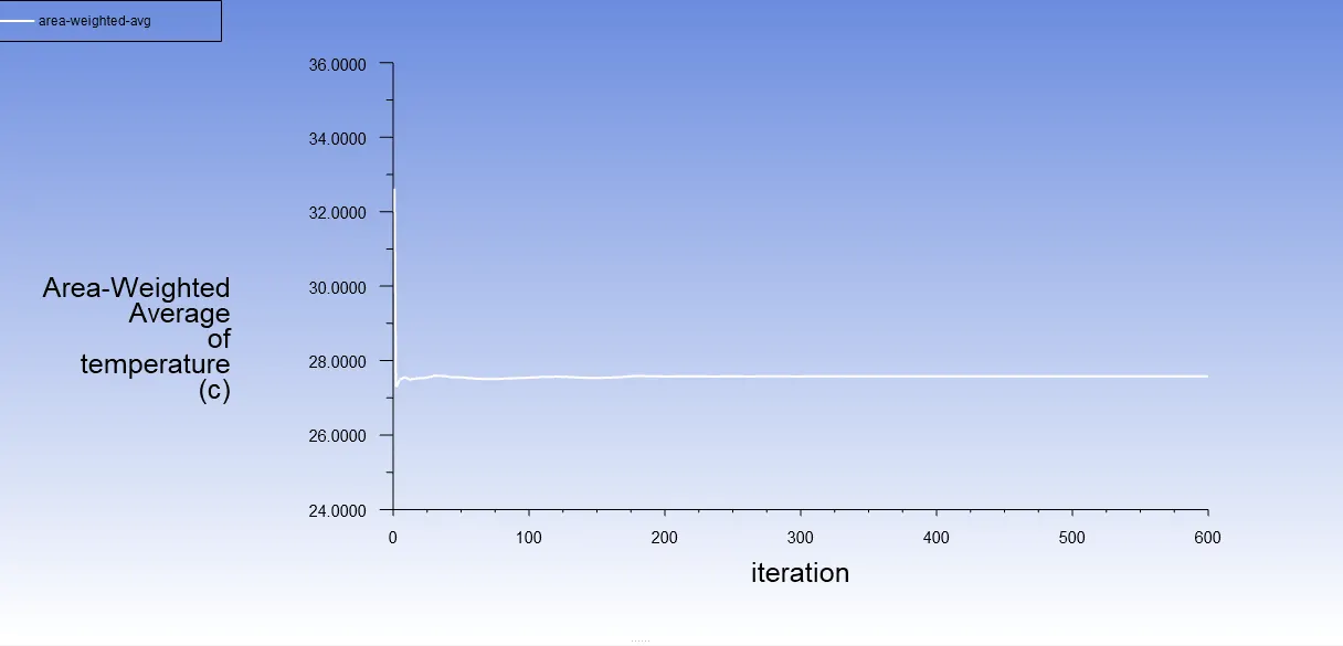
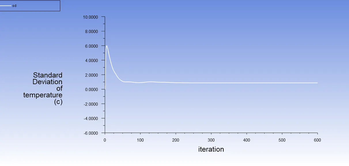
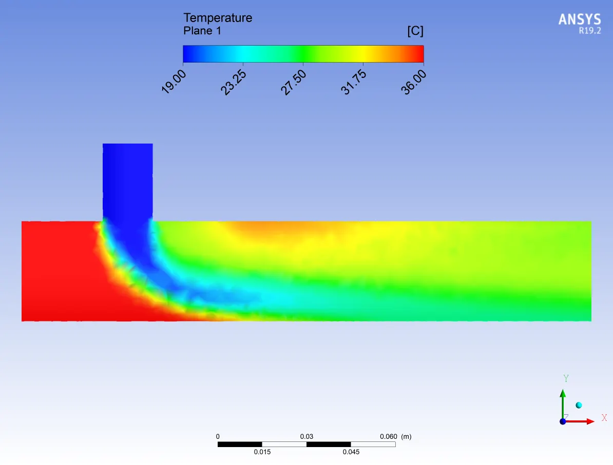
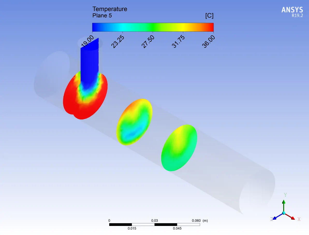
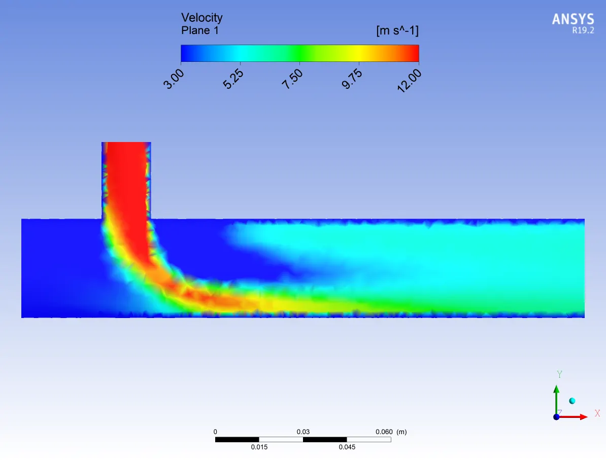
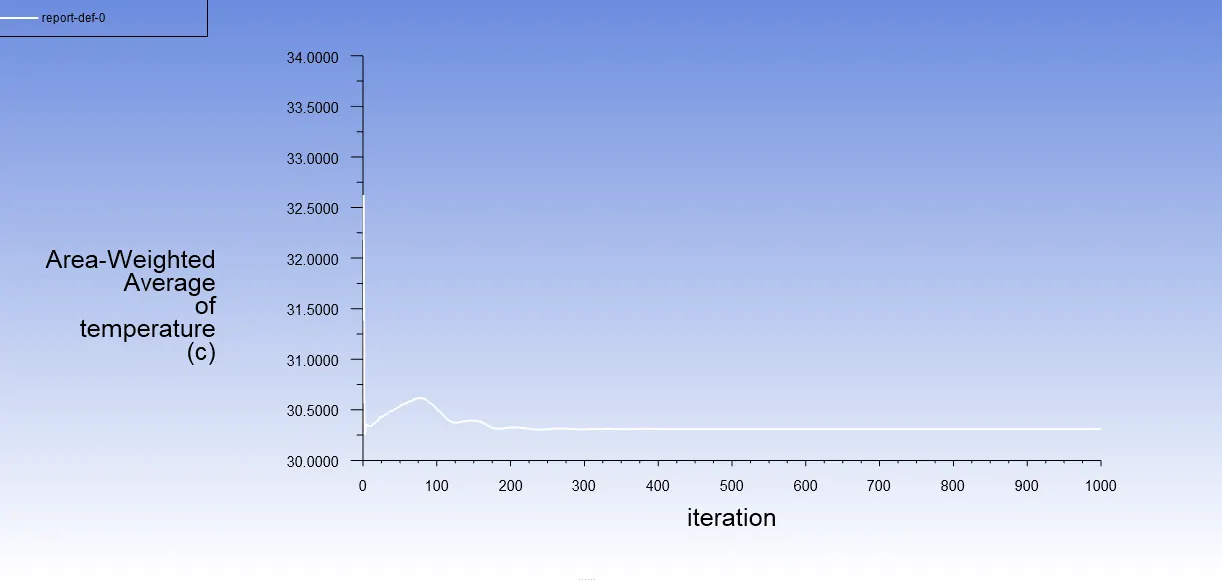
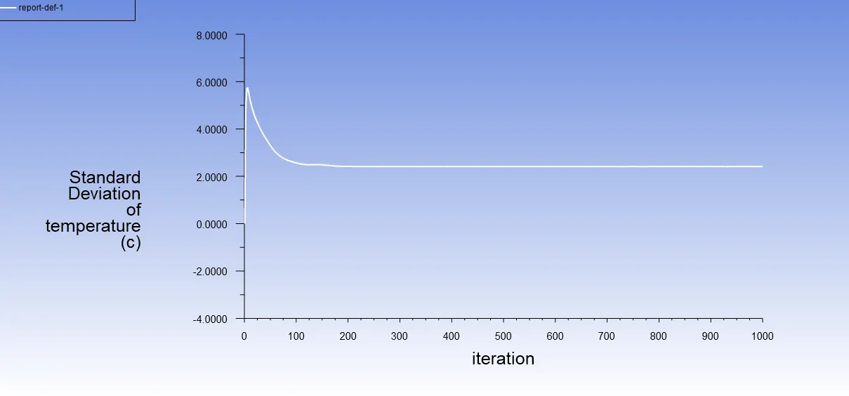
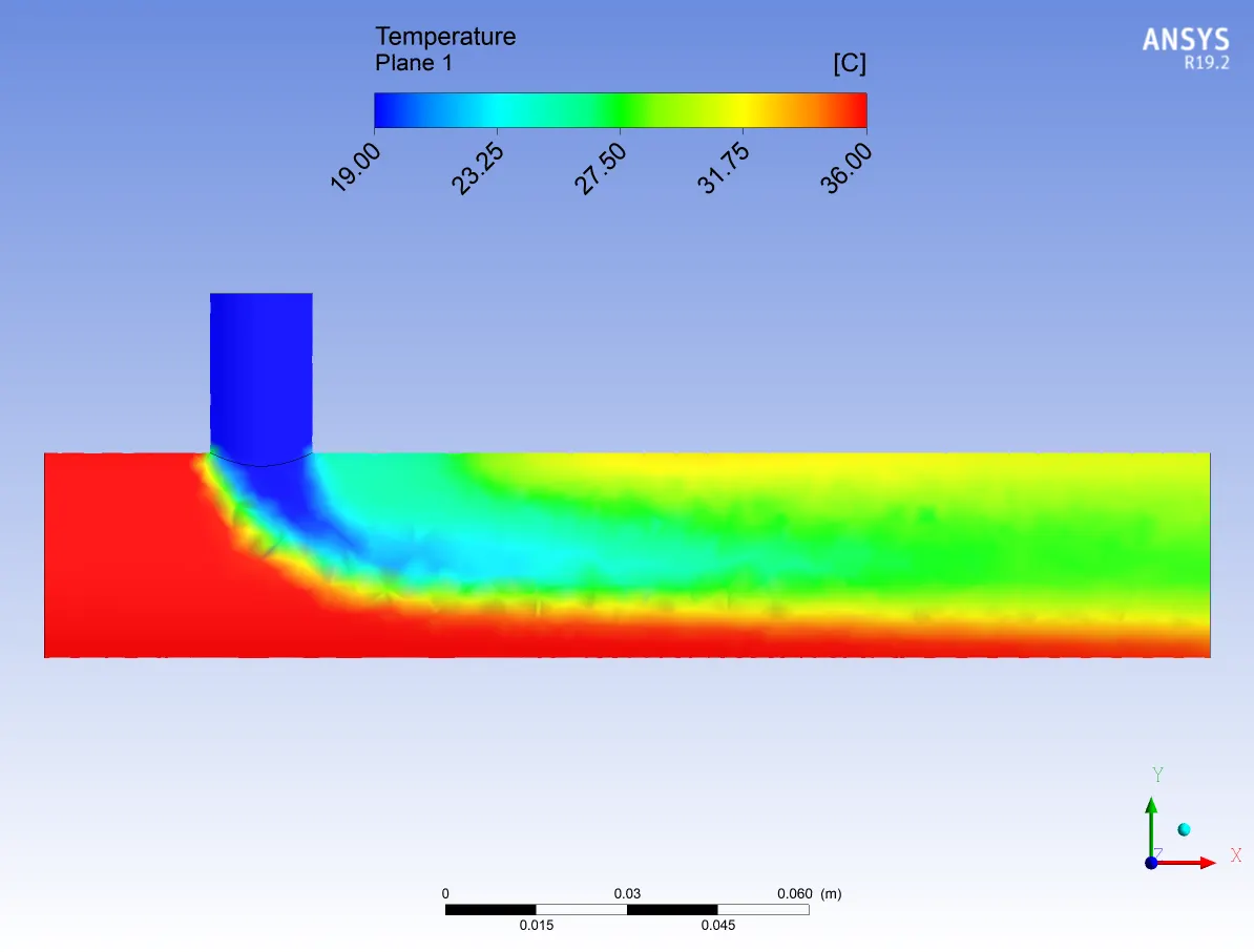
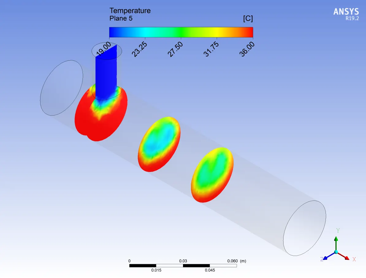
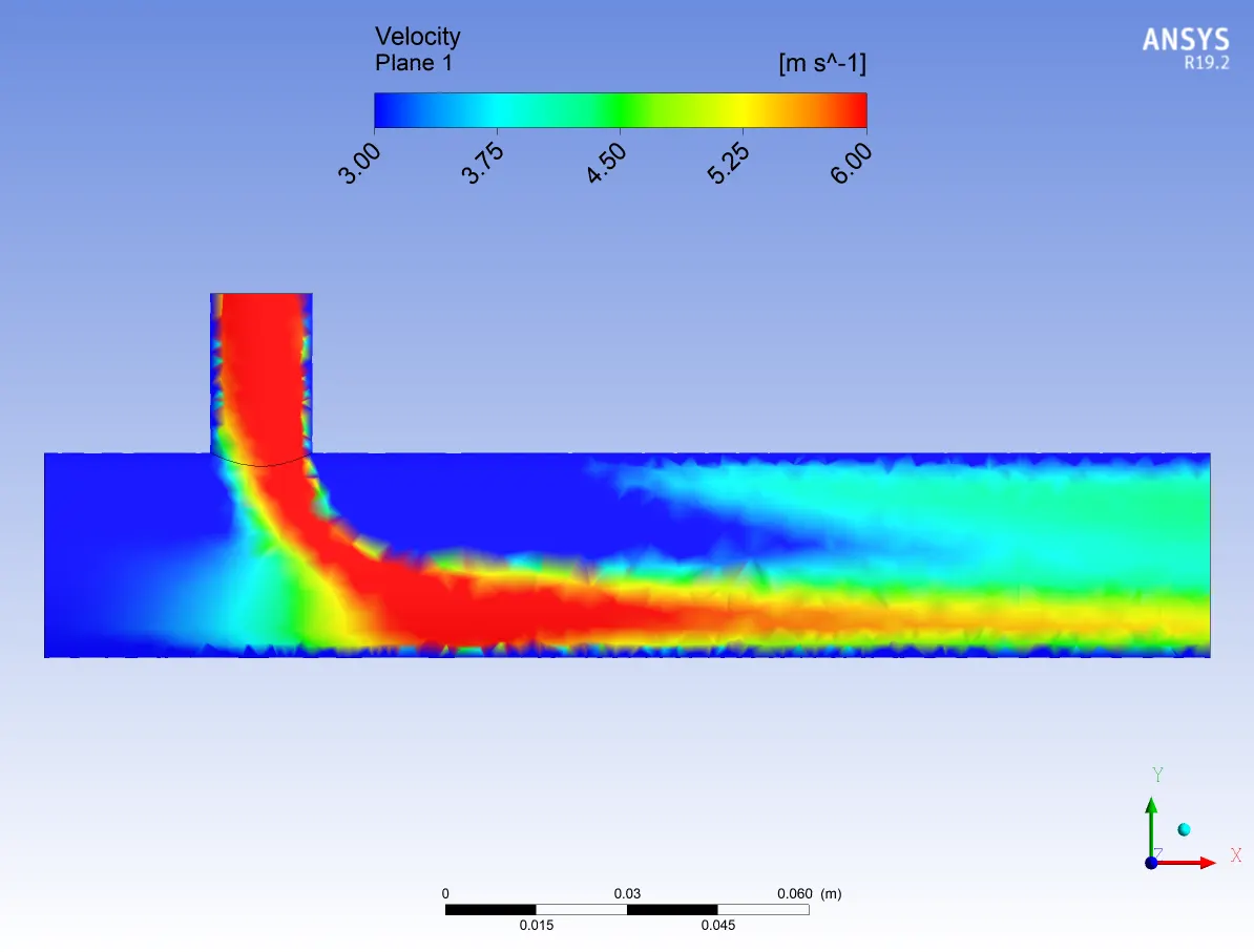
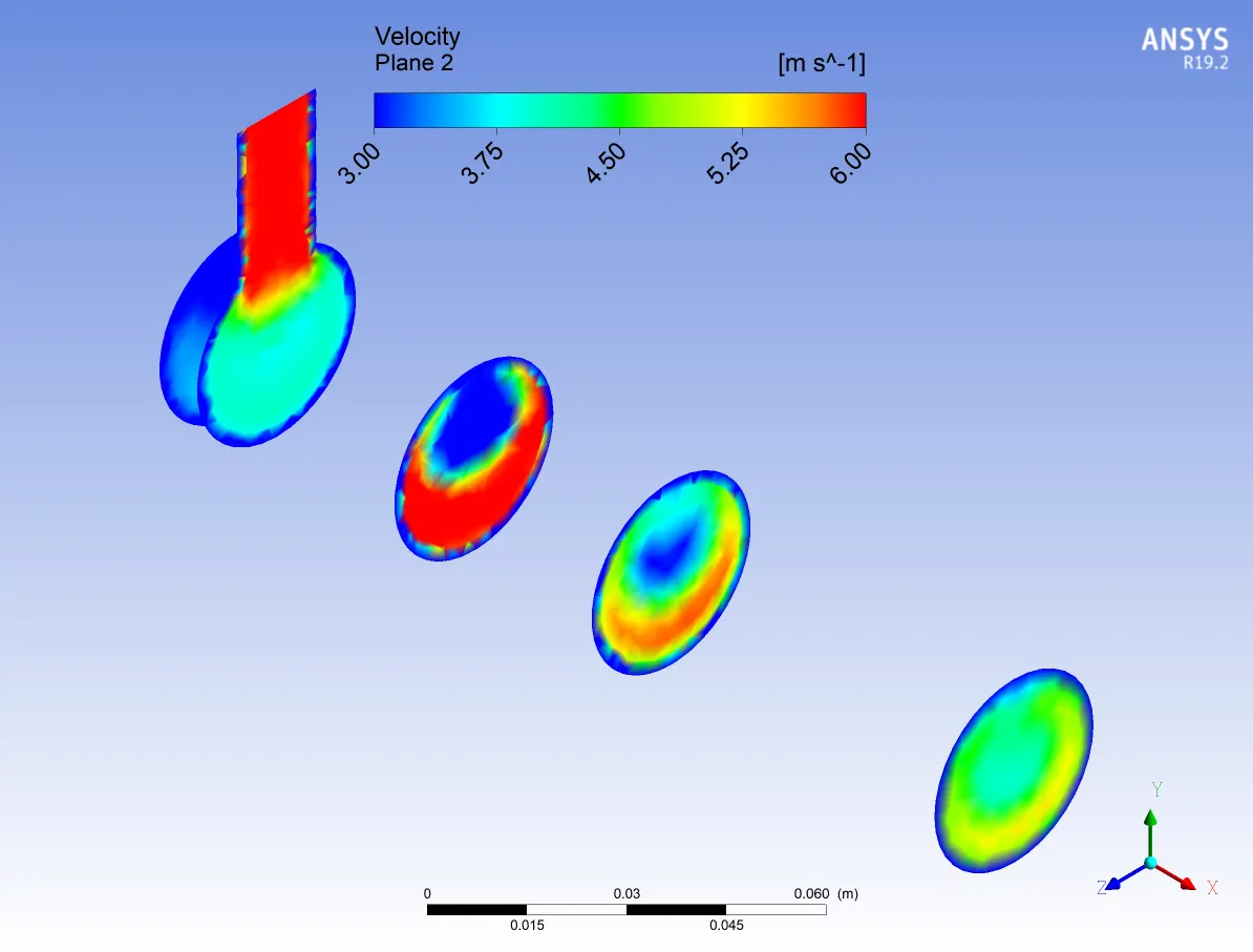
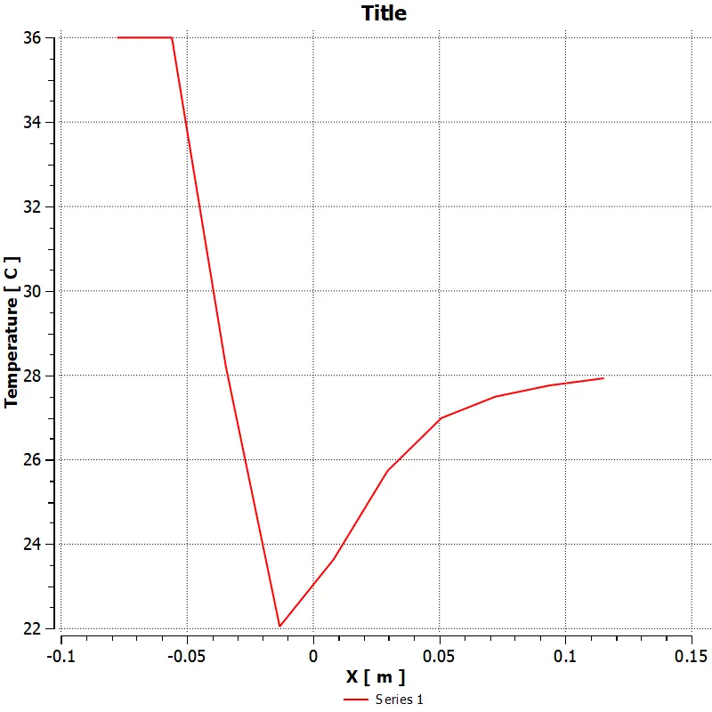
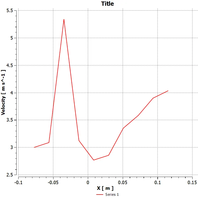
3.k–omega (k–ω) model with momentum ratio 2 :

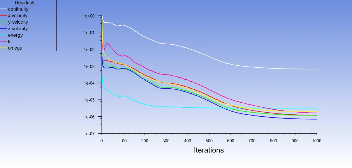
convergence plot	Area weighted average(°C) plot
Standard deviation of temperature(°C) Plot	Temperature contour plot along the pipe
Temperature contour plot across the pipe	Velocity contour plot along the pipe
Velocity contour plot across the pipe	Temperature line plot along the length of the pipe
Velocity line plot along the length of the pipe	Temperature and Velocity contour plot at the outlet
Temperature line plot across the length of the pipe	Velocity line plot across the length of the pipe

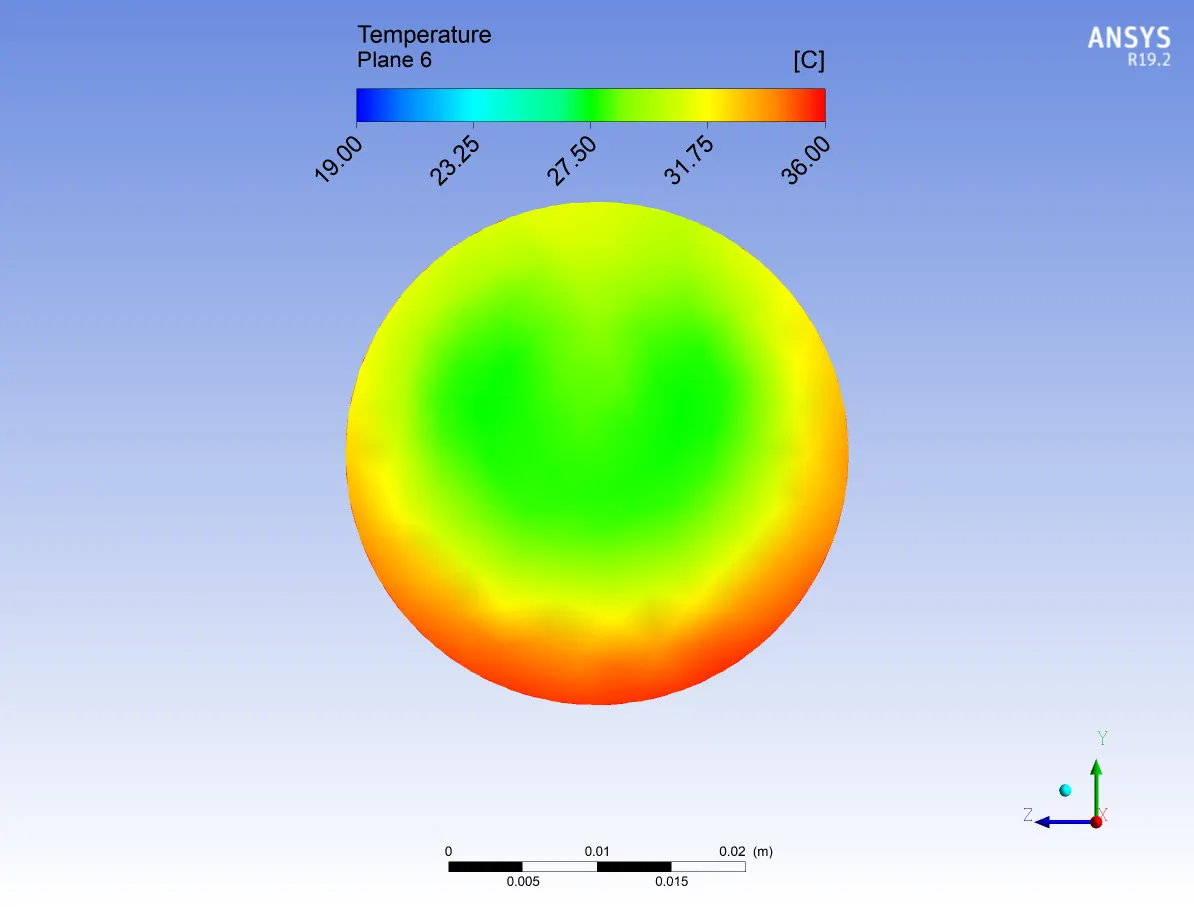
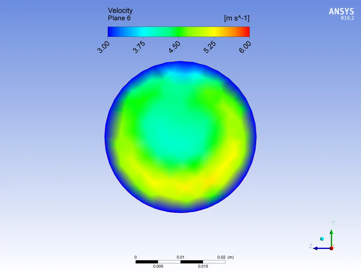
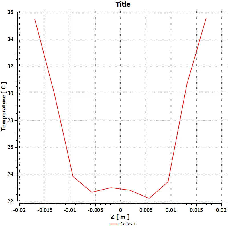
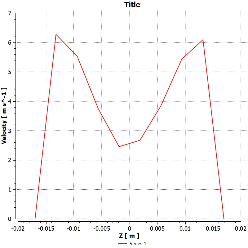
4.k–omega (k–ω) model with momentum ratio 4 :

convergence plot	Area weighted average(°C) plot
Standard deviation of temperature(°C) Plot	Temperature contour plot along the pipe
Temperature contour plot across the pipe	Velocity contour plot along the pipe
Velocity contour plot across the pipe	Temperature line plot along the length of the pipe
Velocity line plot along the length of the pipe	Temperature and Velocity contour plot at the outlet
Temperature line plot across the length of the pipe	Velocity line plot across the length of the pipe

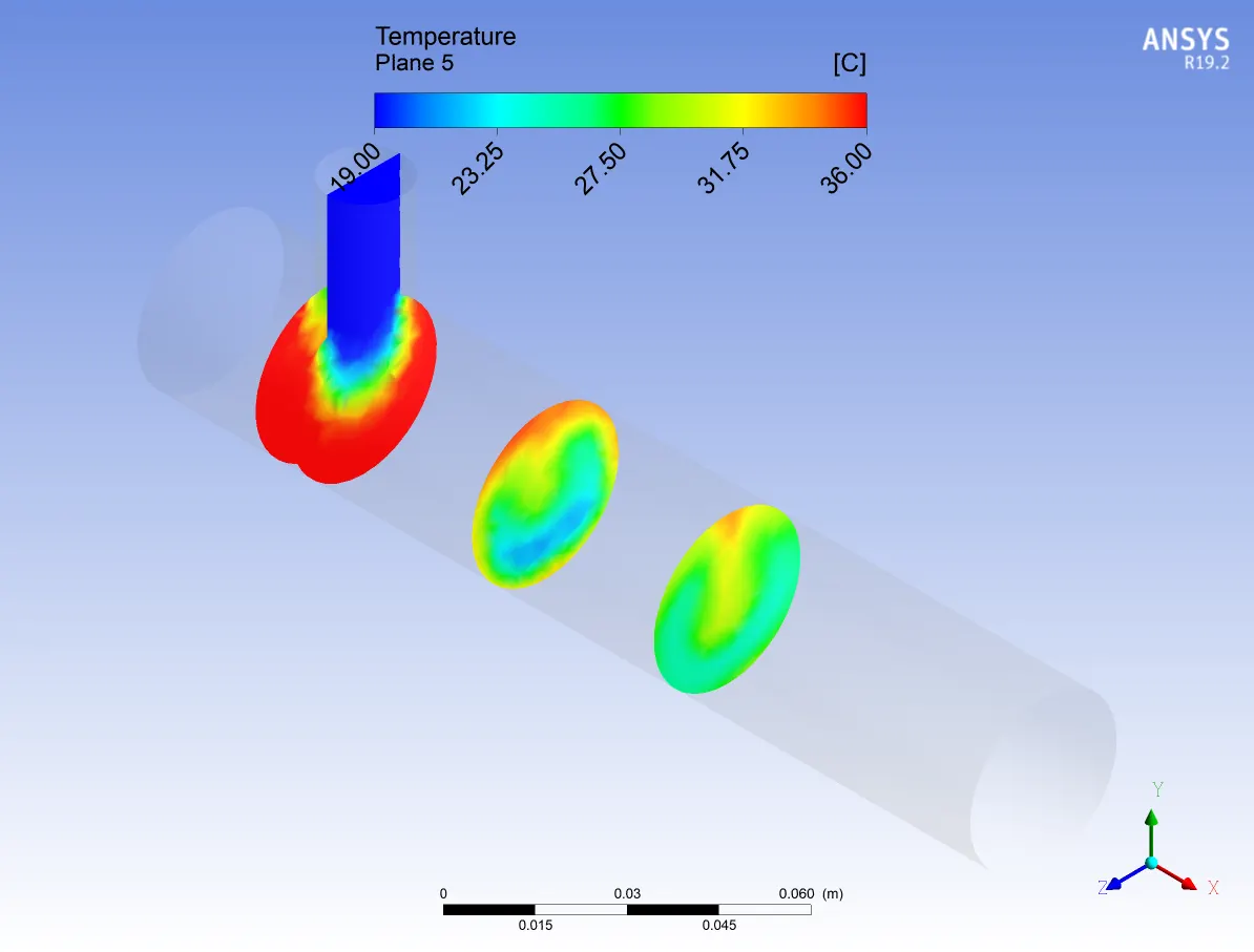
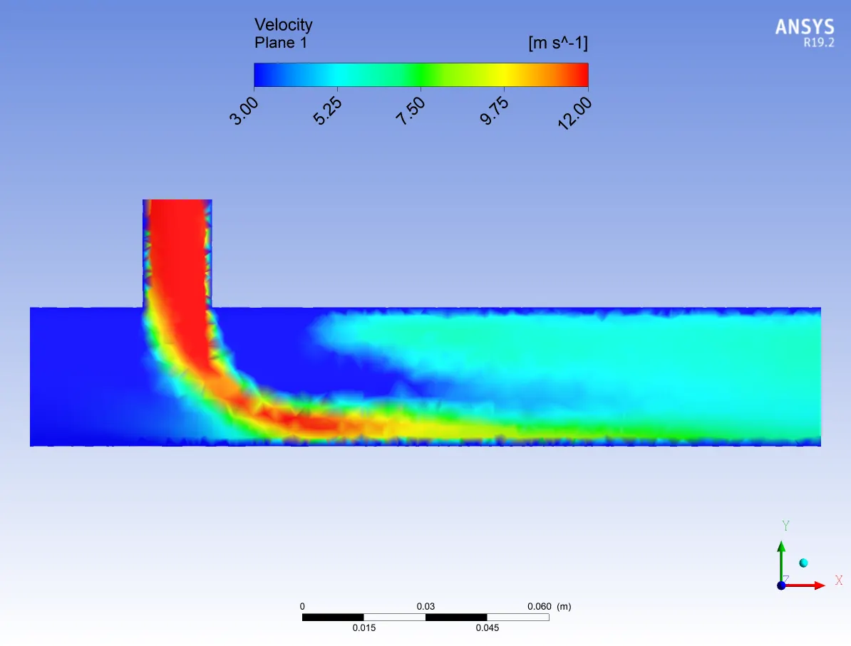
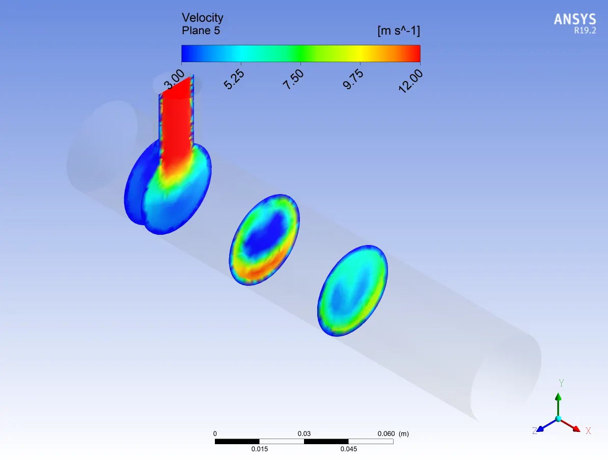
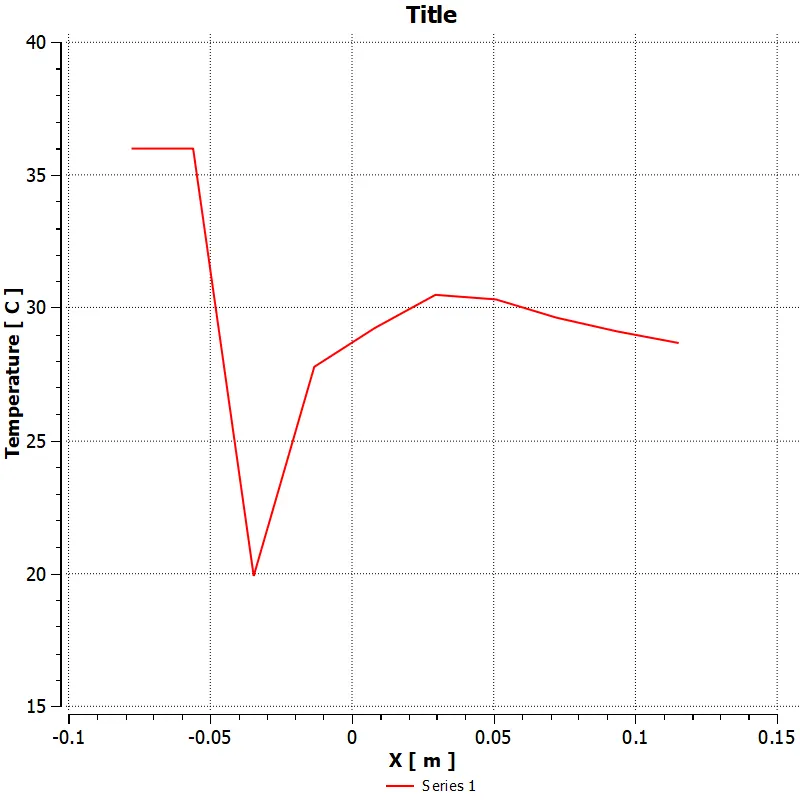
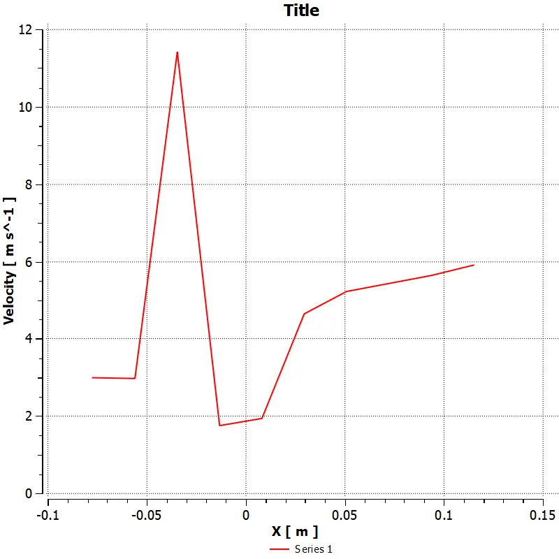
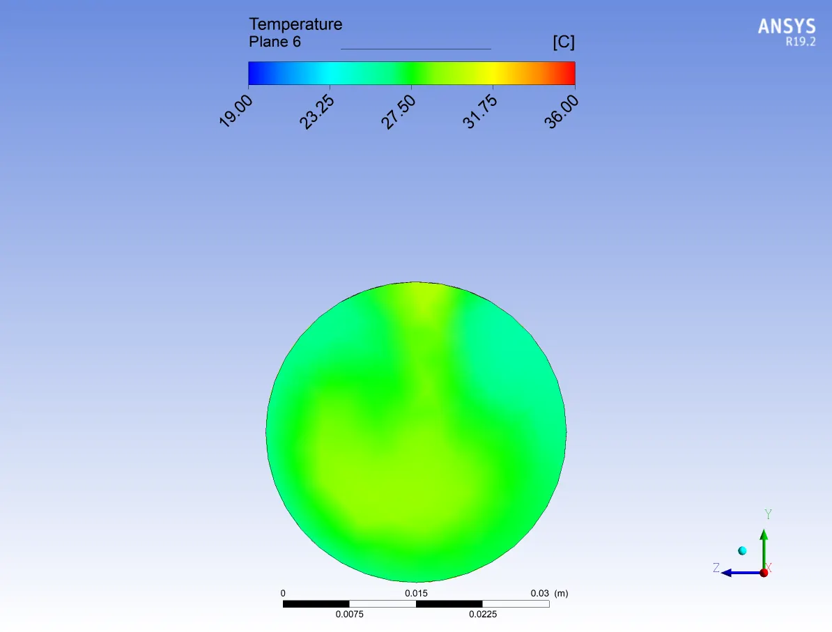
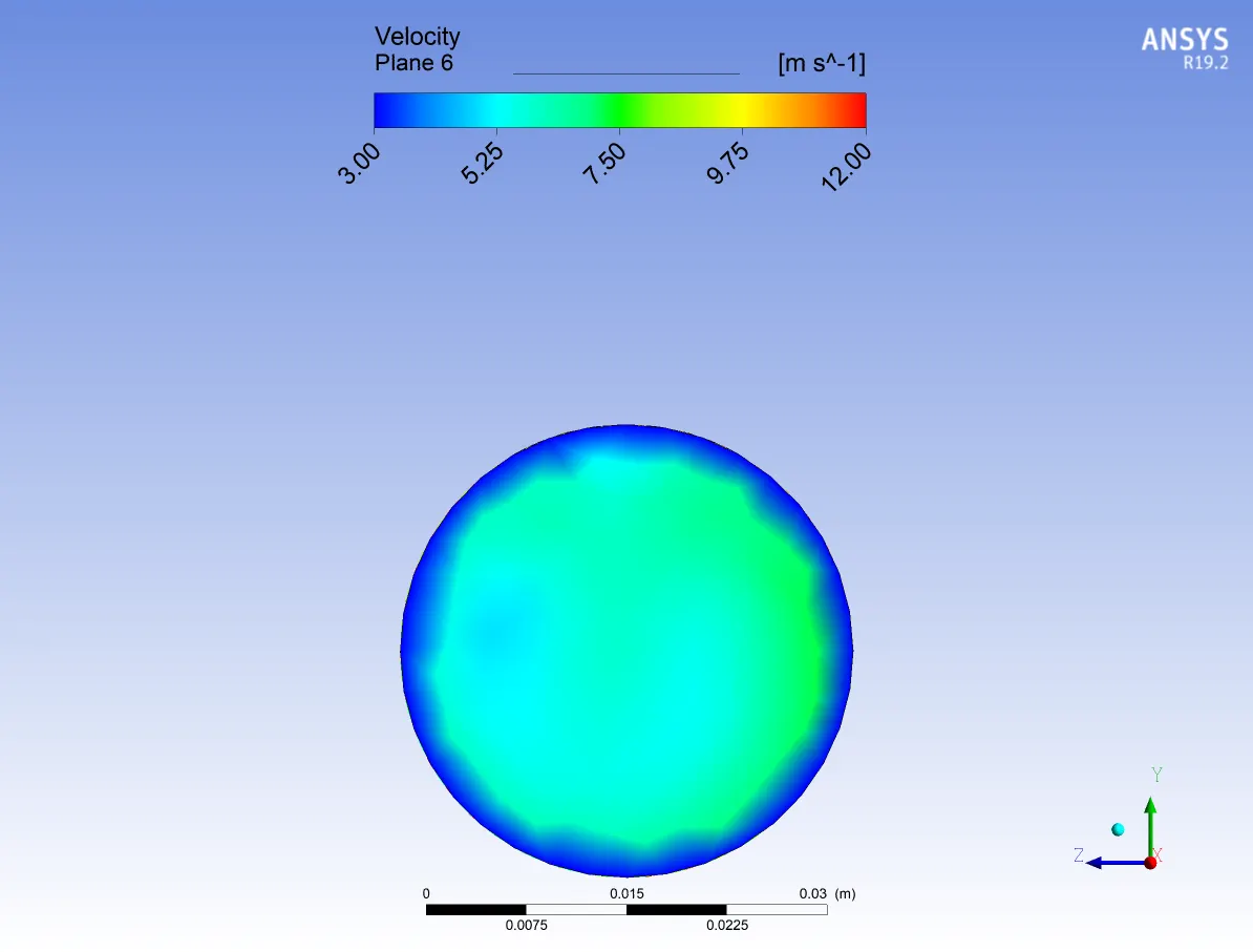
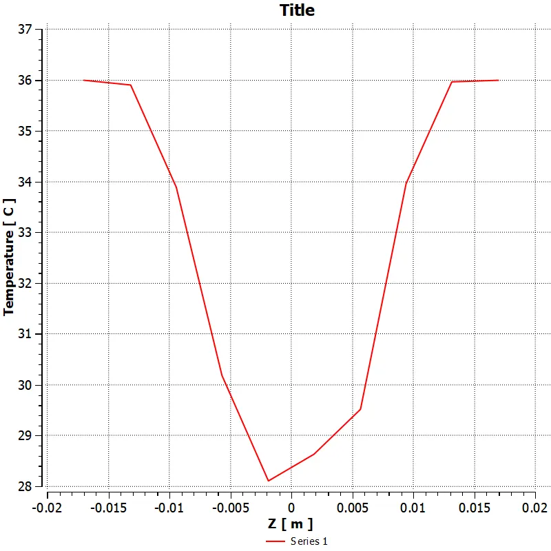
For Short mixing tee with an element size of 3mm :

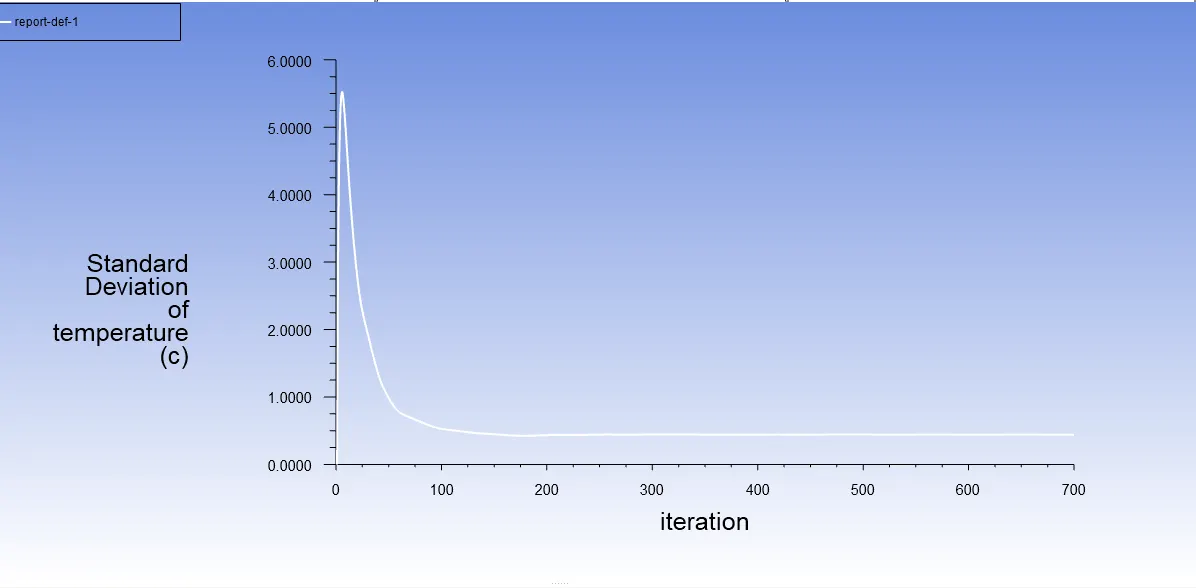
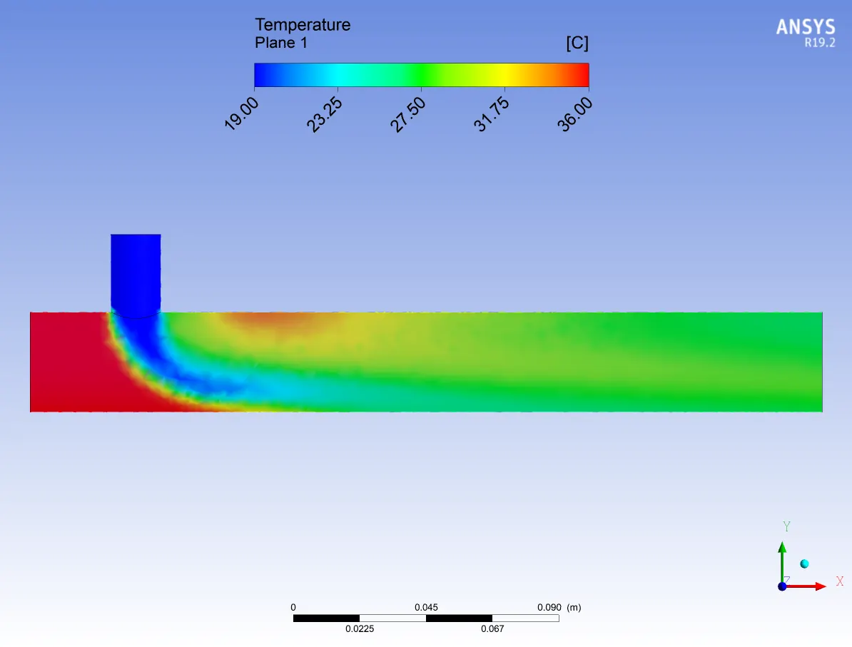
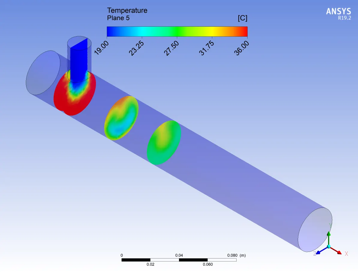
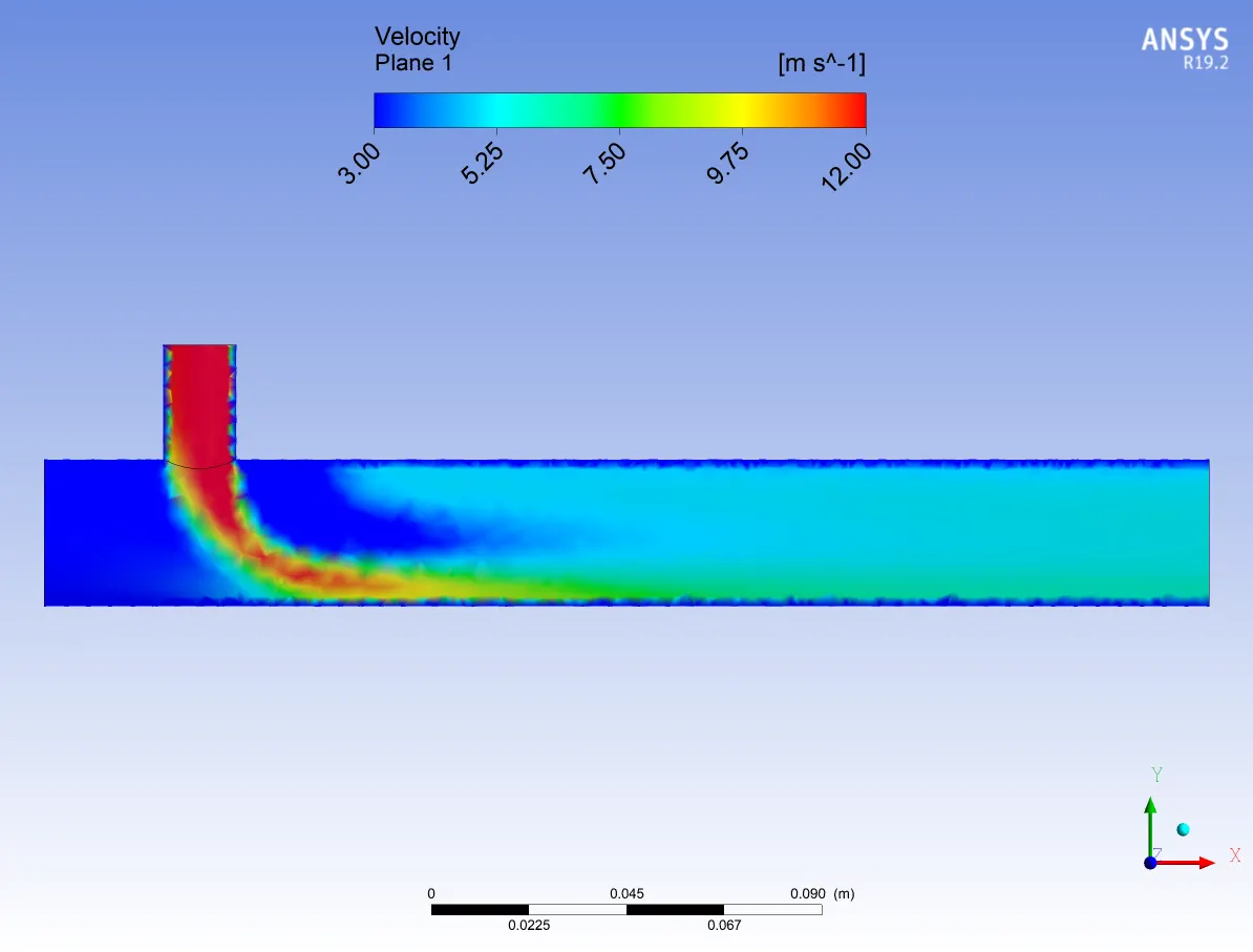
From the above table, it is clear that for the same momentum ratio the standard deviation of temperature is more for k–omega (k–ω) SST model. Higher Standard deviation means the mixing is bad, whereas low standard deviation means that the mixing is good. Since the standard deviation of temperature is less for the K-epsilon (k-ε) model, it has better mixing effectiveness.

Case 2: Long mixing tee

Now we know that the K-epsilon (k-ε) model provides better mixing result. So for the long mixing tee, we will use the K-epsilon (k-ε) turbulence model.

K-epsilon (k-ε) model with momentum ratio 2 :

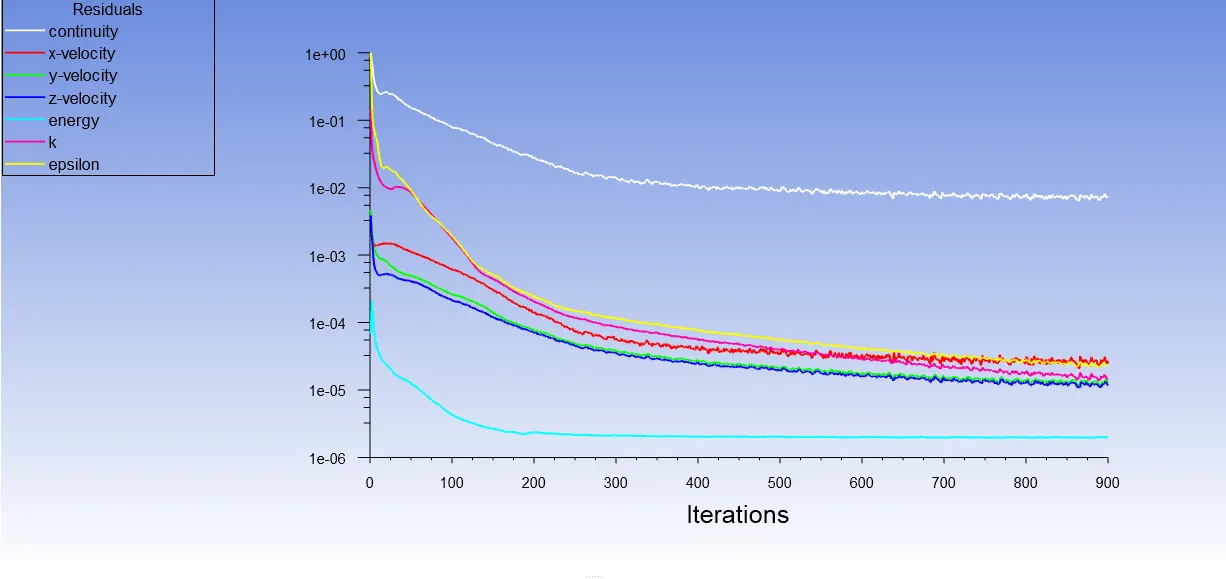
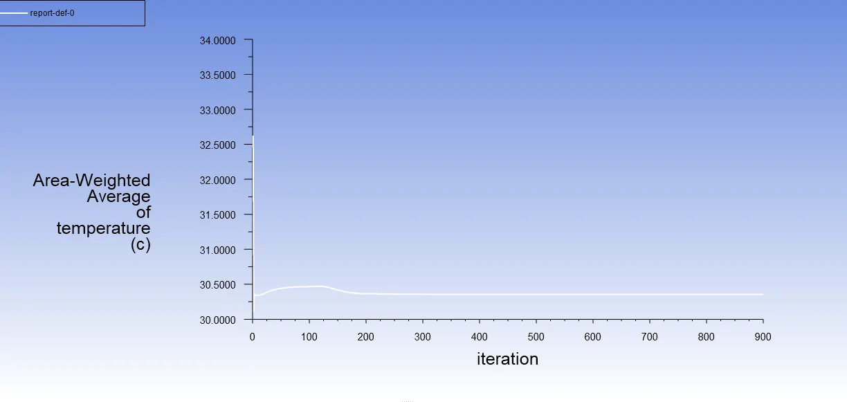
Convergence plot	Area weighted average of temperature(°C)plot
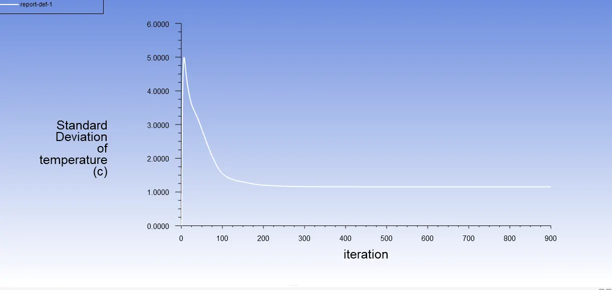
Standard deviation of temperature(°C) Plot	Temperature contour plot along the pipe
Temperature contour plot across the pipe	velocity contour plot along the pipe
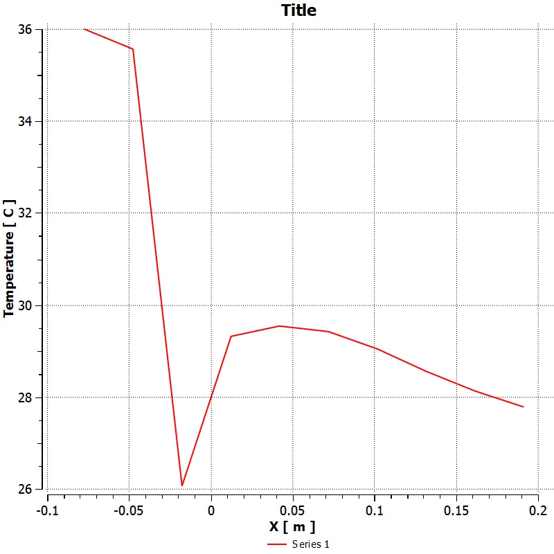
velocity contour plot across the pipe	Temperature line plot along the length of the pipe
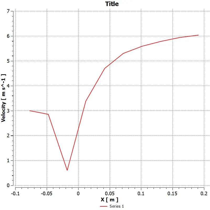
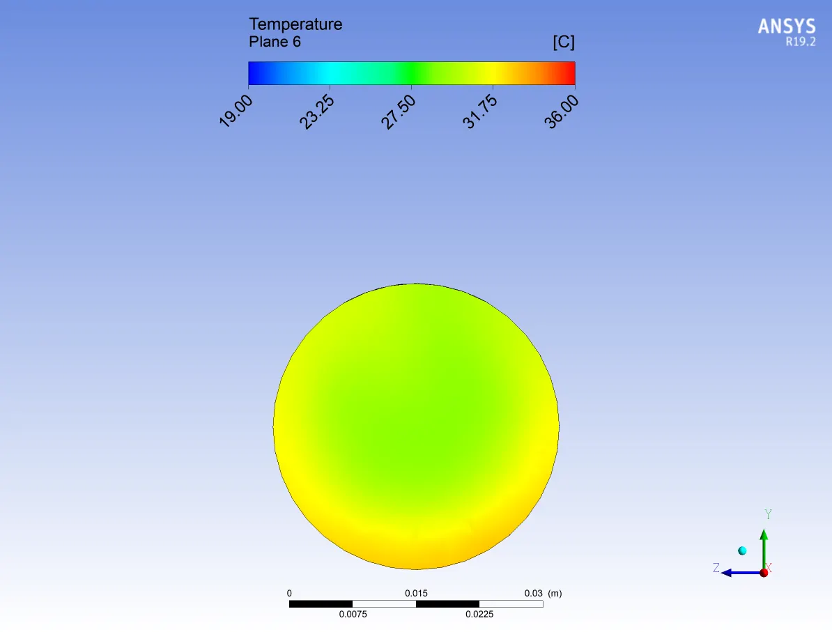
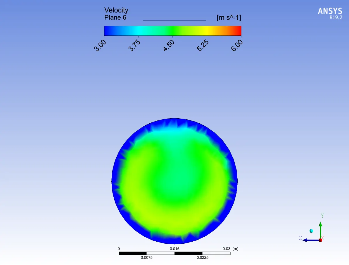
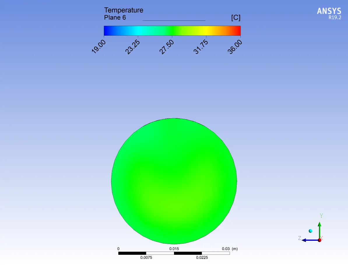
Velocity line plot along the length of the pipe	n Temperature and Velocity contour plot at the outlet
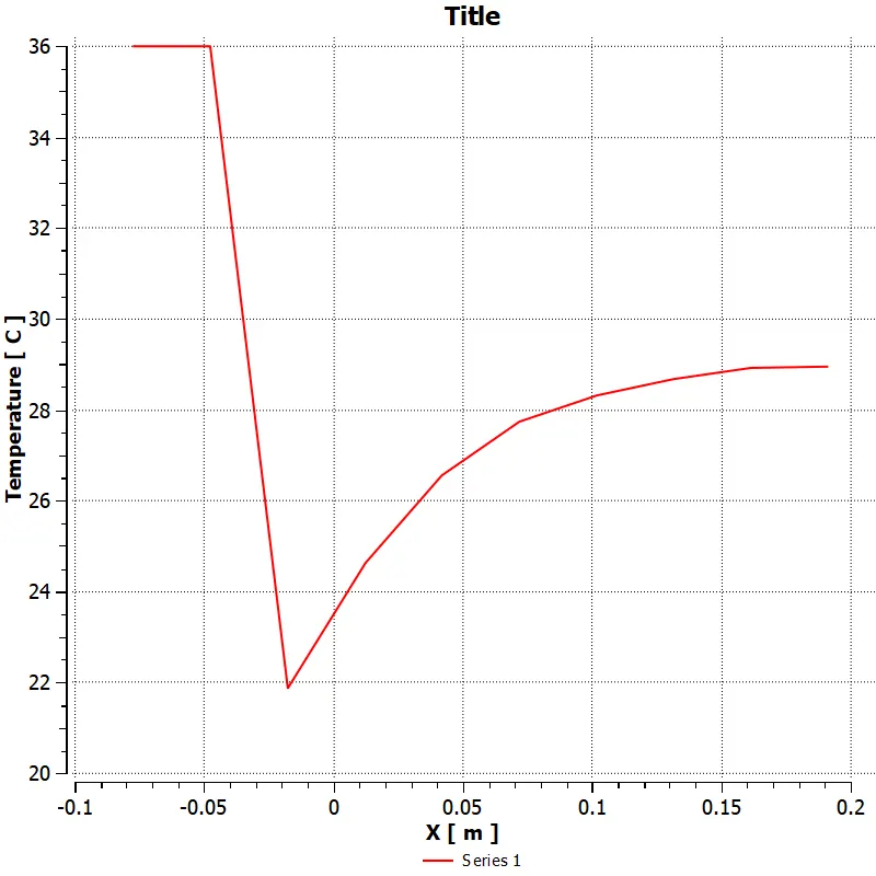
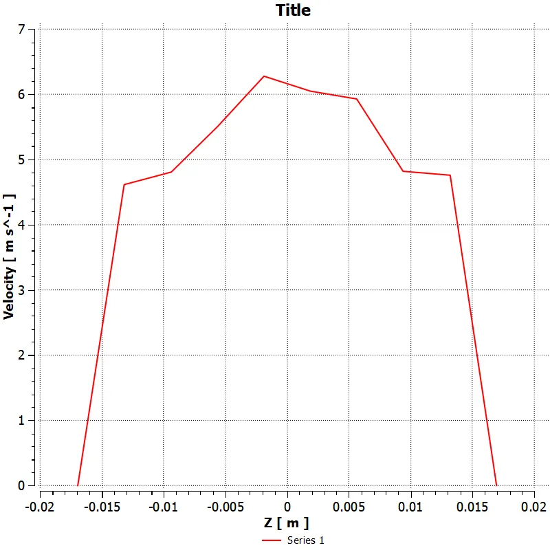
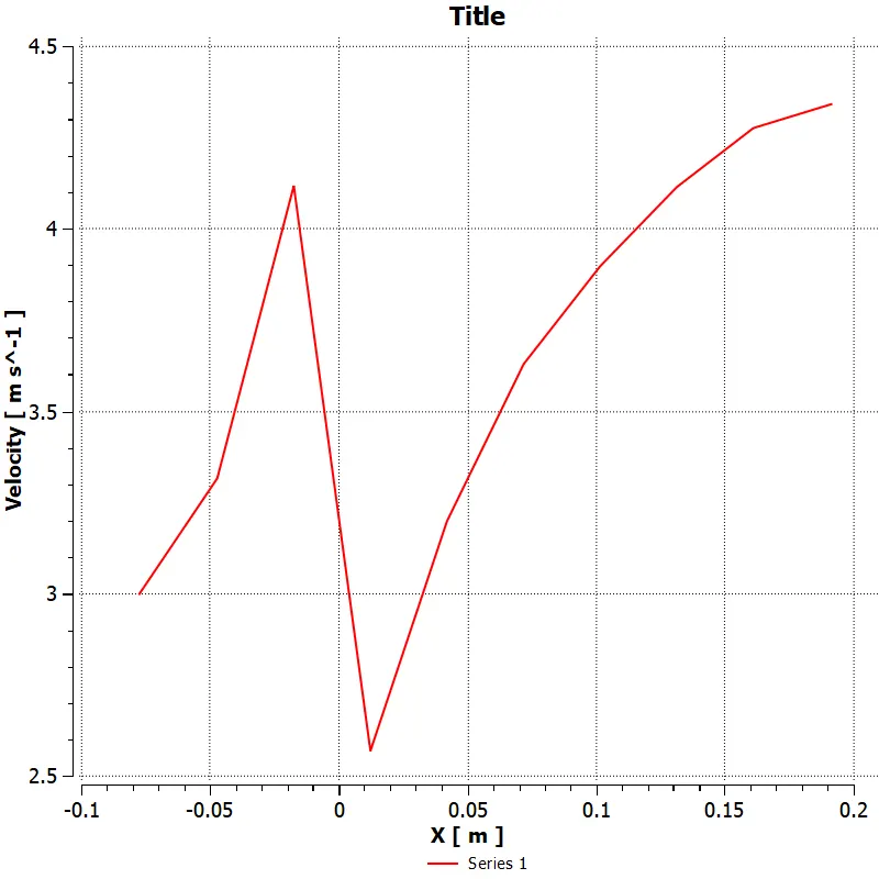
Temperature line plot across the length of the pipe	Velocity line plot across the length of the pipe

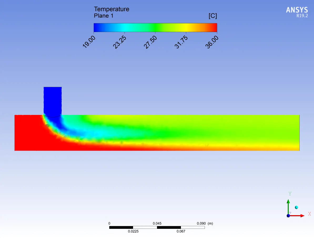
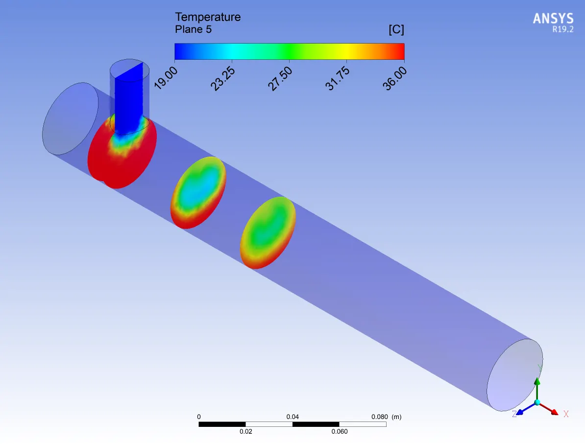
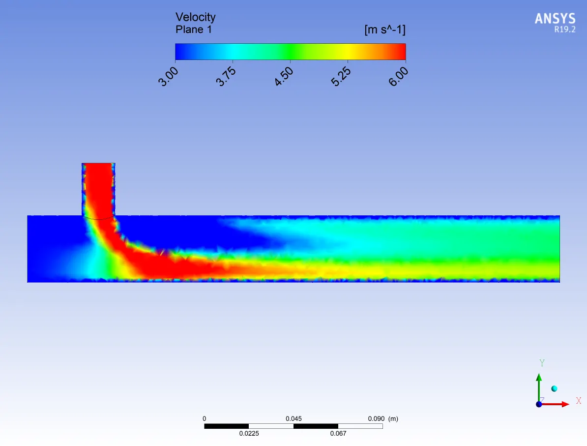
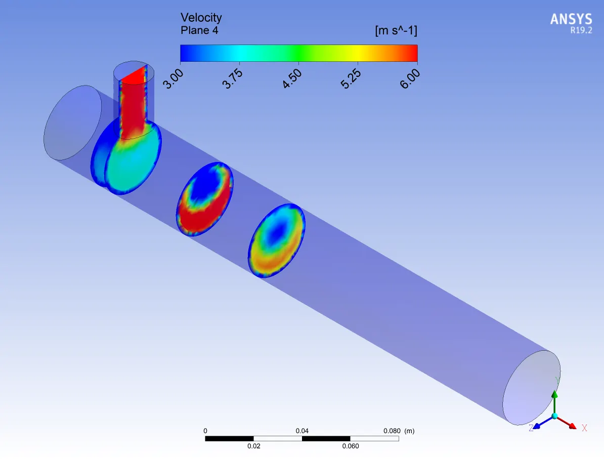
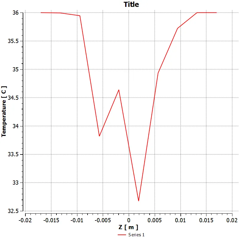
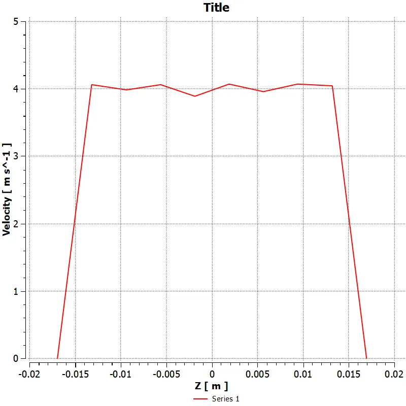
2.K-epsilon (k-ε) model with momentum ratio 4 :

Convergence plot	Area weighted average of temperature(°C)plot
Standard deviation of temperature(°C) Plot	Temperature contour plot along the pipe
Temperature contour plot across the pipe	velocity contour plot along the pipe
Velocity contour plot across the pipe	Temperature line plot along the length of the pipe
velocity line plot along the length of the pipe	Temperature and Velocity contour plot at the outlet
Temperature line plot across the length of the pipe	velocity line plot across the length of the pipe

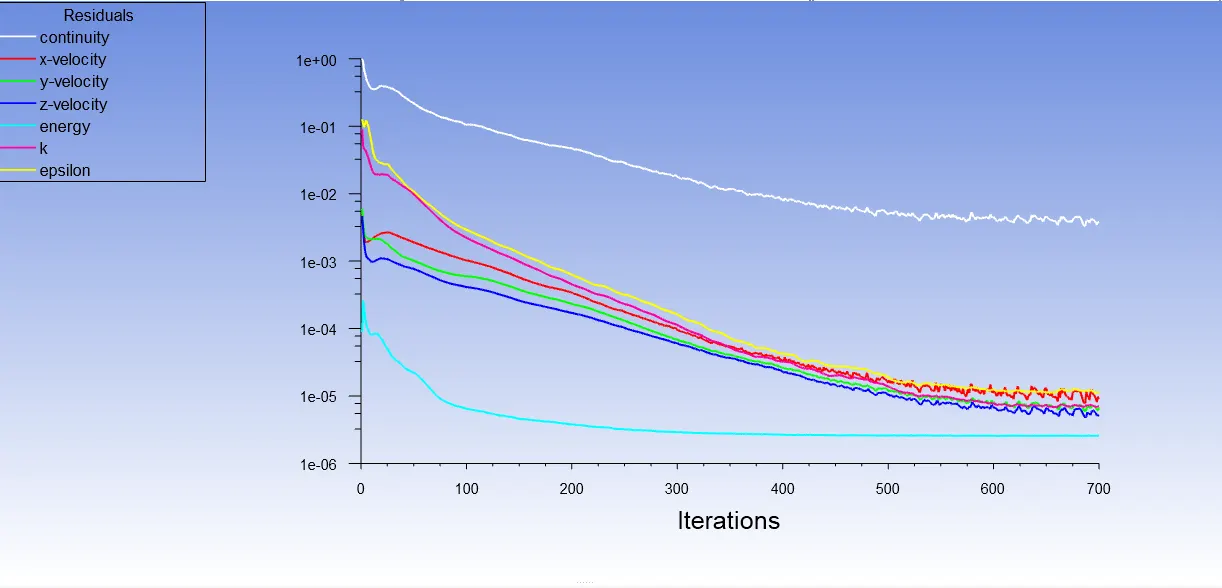
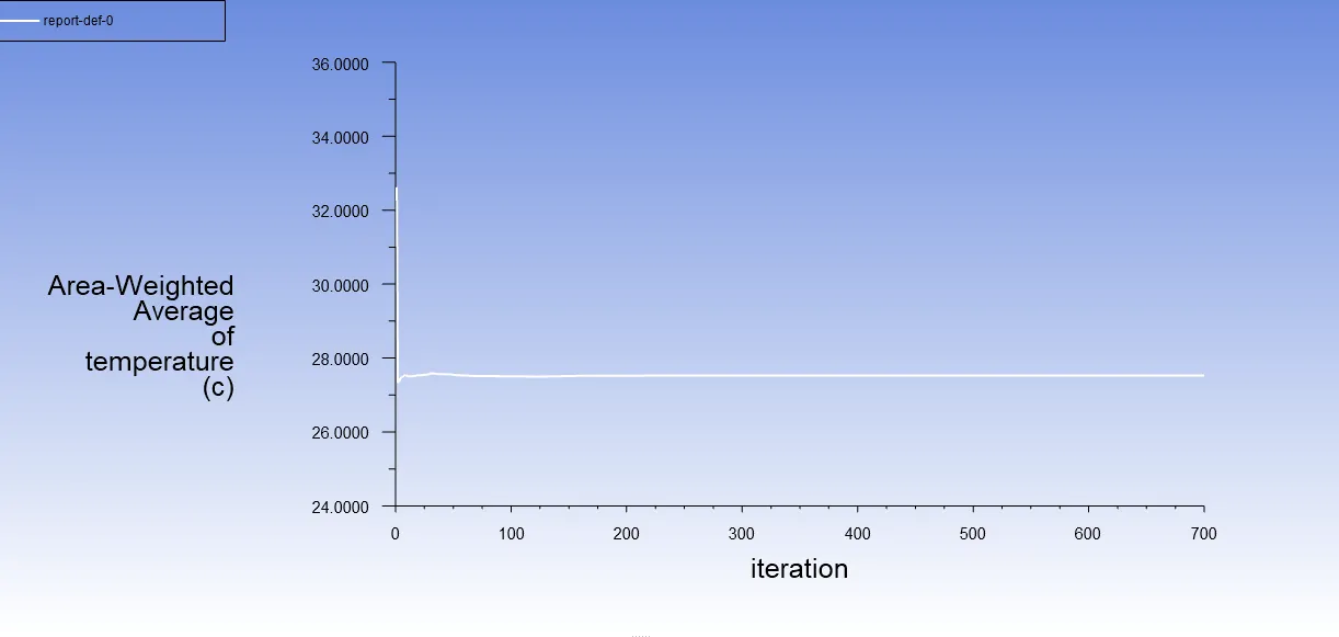
table(b)

--------------------------------------------------------------------------------------------------------------------------------------------------------------------------------------------------------------------------------------------

Mesh independent study :

we will Perform Mesh independent study for second case i.e Long mixing tee.

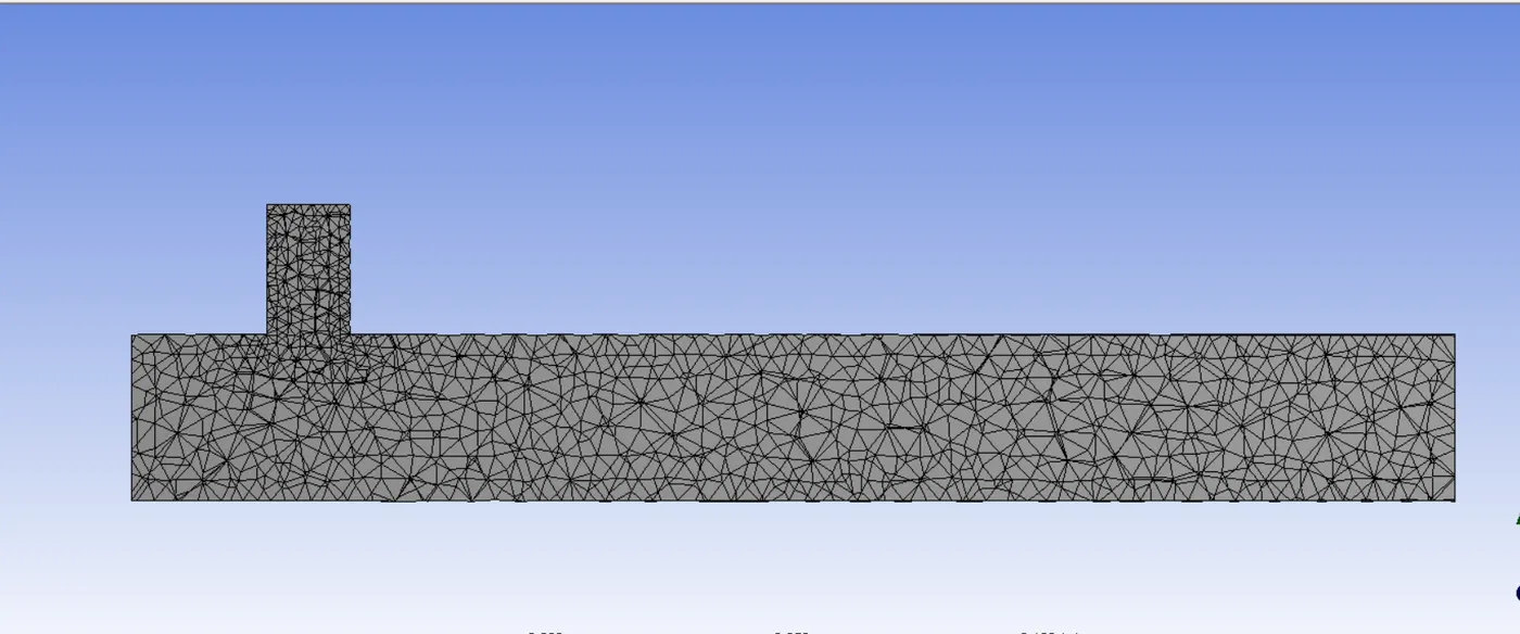
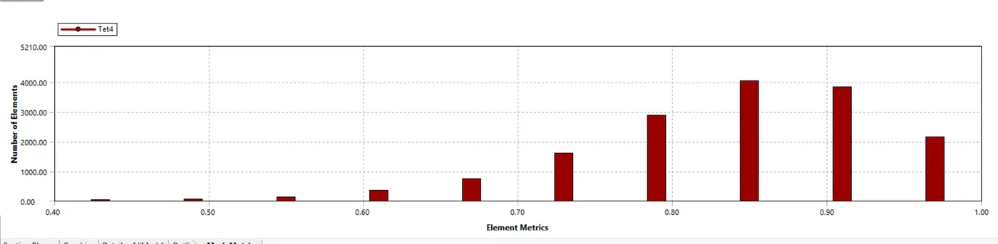
• Mesh element size: 7mm.

Nodes:3499 Elements:15689

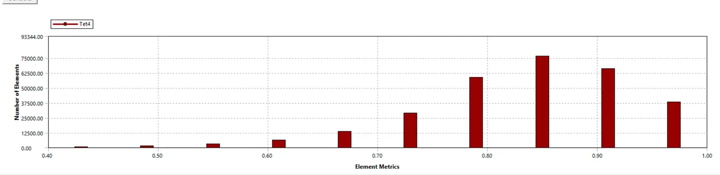
The Mesh matric that identifies elements according to their quality was employed and it can be seen that the elements of lowest quality are minimal, most of the elements have very high quality in the range of 0.75-1.

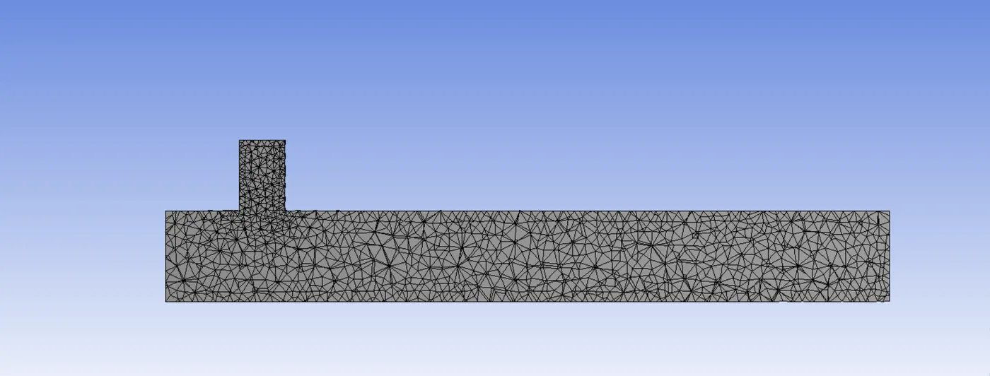
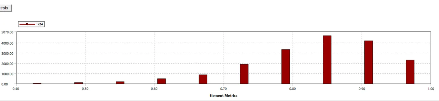
• Mesh element size: 5mm.

Nodes:3958 Elements:17893

The Mesh matric that identifies elements according to their quality was employed and it can be seen that the elements of lowest quality are minimal, most of the elements have very high quality in the range of 0.75-1.

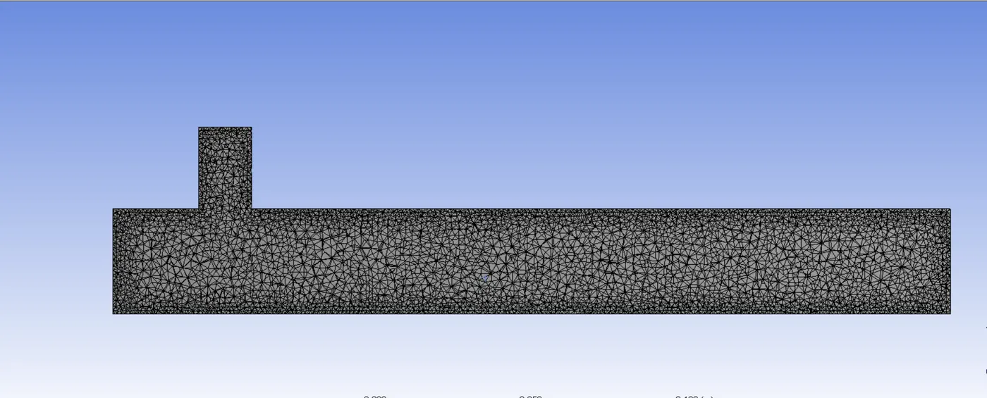
• Mesh element size: 3mm.

Nodes:11802 Elements:57153

The Mesh matric that identifies elements according to their quality was employed and it can be seen that the elements of lowest quality are minimal, most of the elements have very high quality in the range of 0.8-1.

• Mesh element size: 1.5mm

Nodes:57291 Elements:291410

The Mesh matric that identifies elements according to their quality was employed and it can be seen that the elements of lowest quality are minimal, most of the elements have very high quality in the range of 0.8-1.

Convergence plots of case 2 with momentum ratio 4 using the K-epsilon turbulence model :

For Mesh element size: 7mm Number of iterations for convergence: 275	For Mesh element size: 5mm Number of iterations for convergence: 300
For Mesh element size: 3mm Number of iterations for convergence: 550	For Mesh element size:1.5mm Number of iterations for convergence: 1000

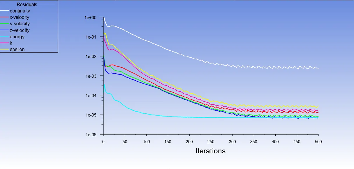
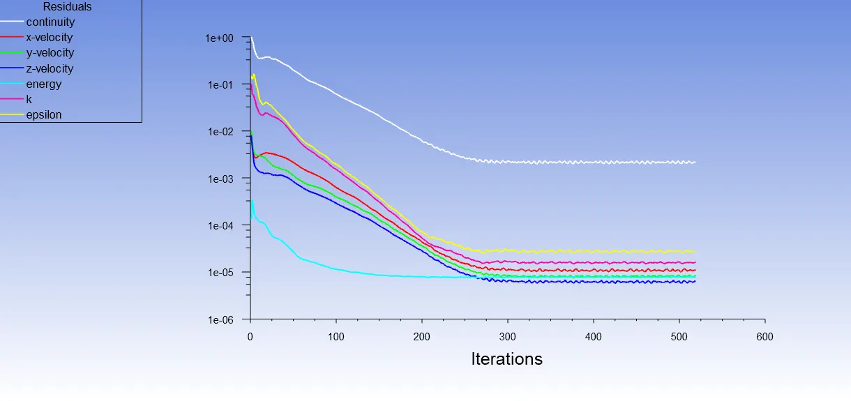
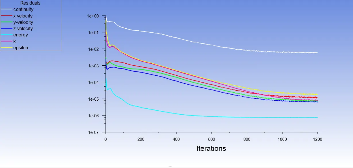
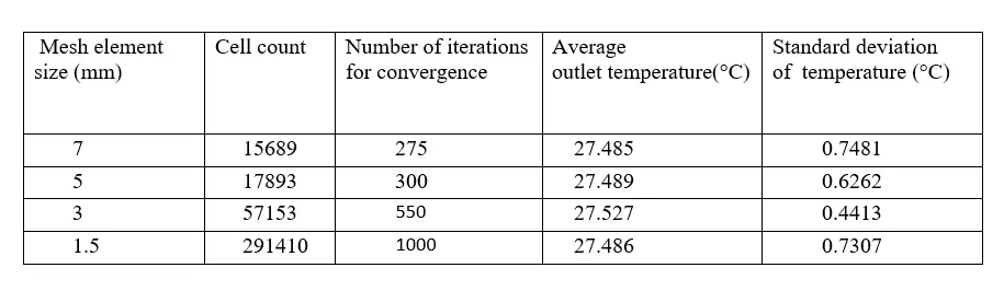
From the above table, for the mesh with an element size of 5mm and 1.5mm, the difference between Average outlet temperature is negligible. So the mesh with an element size of 5mm and 1.5mm will be coarse mesh and fine mesh respectively. For mesh with an element size of 3mm, the standard deviation of temperature is less when compared with other meshes, it provides the best mixing efficiency.

Conclusion:

The steady-state simulations are carried using ANSYS Fluent for short and long mixing tee for different momentum ratio and it is found that to get good mixing te velocity of chilled air is Very important. By increasing the velocity of chilled air by a factor of 2 we can reduce the outlet temperature from around 30°Cto 27°C.

The longer configuration results are similar to that of shorter configuration. So increasing length is not helpful. When we increase the velocity we get better turbulent mixing. Majority of the mixing occurs because of the higher velocity and as we go along the length of the pipe there is additional mixing due to the diffusion but it is not dominant.

Reference Formulas :